A Gentle Tutorial on Linear Algebra with Python
Published on Thursday, 21-08-2025
(Adopted from CS221)
🔢 A Gentle Tutorial on Linear Algebra with Python
Linear Algebra is the foundation of modern data science, computer graphics, and machine learning. In this tutorial, we’ll walk through key concepts step by step—using notation, Python code, and visualizations to make things clear.
1. Vectors
A vector is an ordered list of numbers. It can represent quantities like position, velocity, or weights in a neural network.
Notation:
Example:
Python:
import numpy as np

# define a vector
v = np.array([2, 3])
print("Vector v:", v)
2. Vector Norm
The norm measures the “length” or “magnitude” of a vector. For vector :
This is the Euclidean norm (L2 norm).
Python:
norm_v = np.linalg.norm(v)
print("Norm of v:", norm_v)
3. Vector Normalization
To normalize a vector, divide it by its norm so its length becomes 1:
Python:
v_normalized = v / np.linalg.norm(v)
print("Normalized v:", v_normalized)
4. Vector Operations
- Addition:
- Scalar Multiplication:
Python:
u = np.array([1, 4])
add = u + v
scalar_mul = 3 * v
print("u + v =", add)
print("3 * v =", scalar_mul)
5. Dot Product
The dot product measures similarity between two vectors:
It’s also related to the angle between vectors:
Python:
dot = np.dot(u, v)
print("u · v =", dot)
6. Matrices
A matrix is a 2D array of numbers:
Python:
A = np.array([[1, 2, 3],
              [4, 5, 6]])
print("Matrix A:\n", A)
7. Matrix-Vector Multiplication
If is a matrix of size and a vector of size :
Example:
Python:
x = np.array([1, 0, -1])
y = A @ x
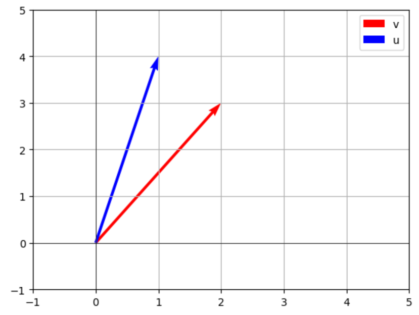
print("A * x =", y)8. Visualizing Vectors
We can visualize 2D vectors using matplotlib:
import matplotlib.pyplot as plt

# plot vectors
origin = [0], [0]  # starting point
plt.quiver(*origin, v[0], v[1], angles='xy', scale_units='xy', scale=1, color='r', label="v")
plt.quiver(*origin, u[0], u[1], angles='xy', scale_units='xy', scale=1, color='b', label="u")

plt.xlim(-1, 5)
plt.ylim(-1, 5)
plt.axhline(0, color='black', linewidth=0.5)
plt.axvline(0, color='black', linewidth=0.5)
plt.grid()
plt.legend()
plt.show()
This will plot u (blue) and v (red) from the origin.
✅ Conclusion
In this tutorial, we covered:
- What vectors are, their norms, and normalization
- Vector operations (addition, scaling, dot product)
- Matrices and matrix-vector multiplication
- Visualizing vectors in 2D
These foundations are essential for deeper topics like linear transformations, eigenvalues, and machine learning applications.