From Linear Classifier to Convolutional Neural Networks

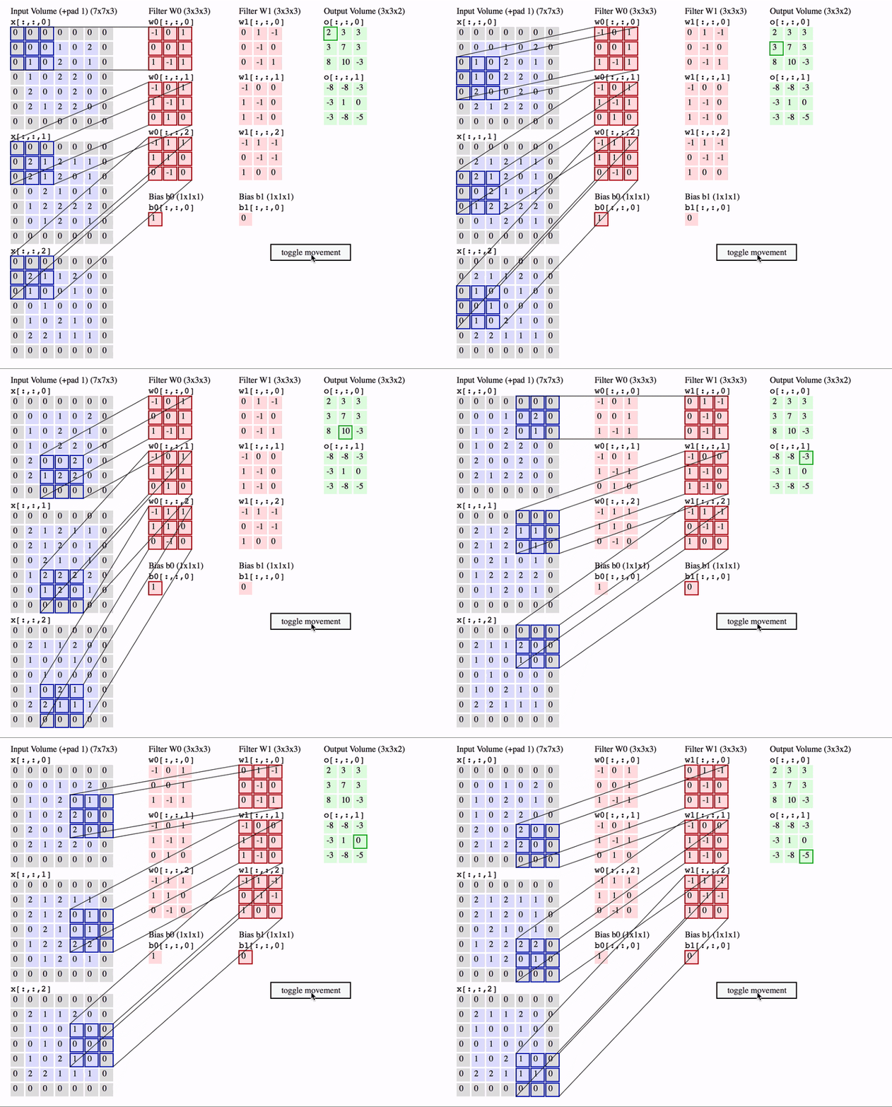
(Adopted from CS231n - Computer Vision with Deep Learning)

Deep Learning is a branch of machine learning that uses neural networks with multiple layers to learn representations of data with multiple levels of abstraction. One of the most common applications of deep learning is in image classification, where the goal is to categorize images into different classes.

Image Classification with Linear Classifiers

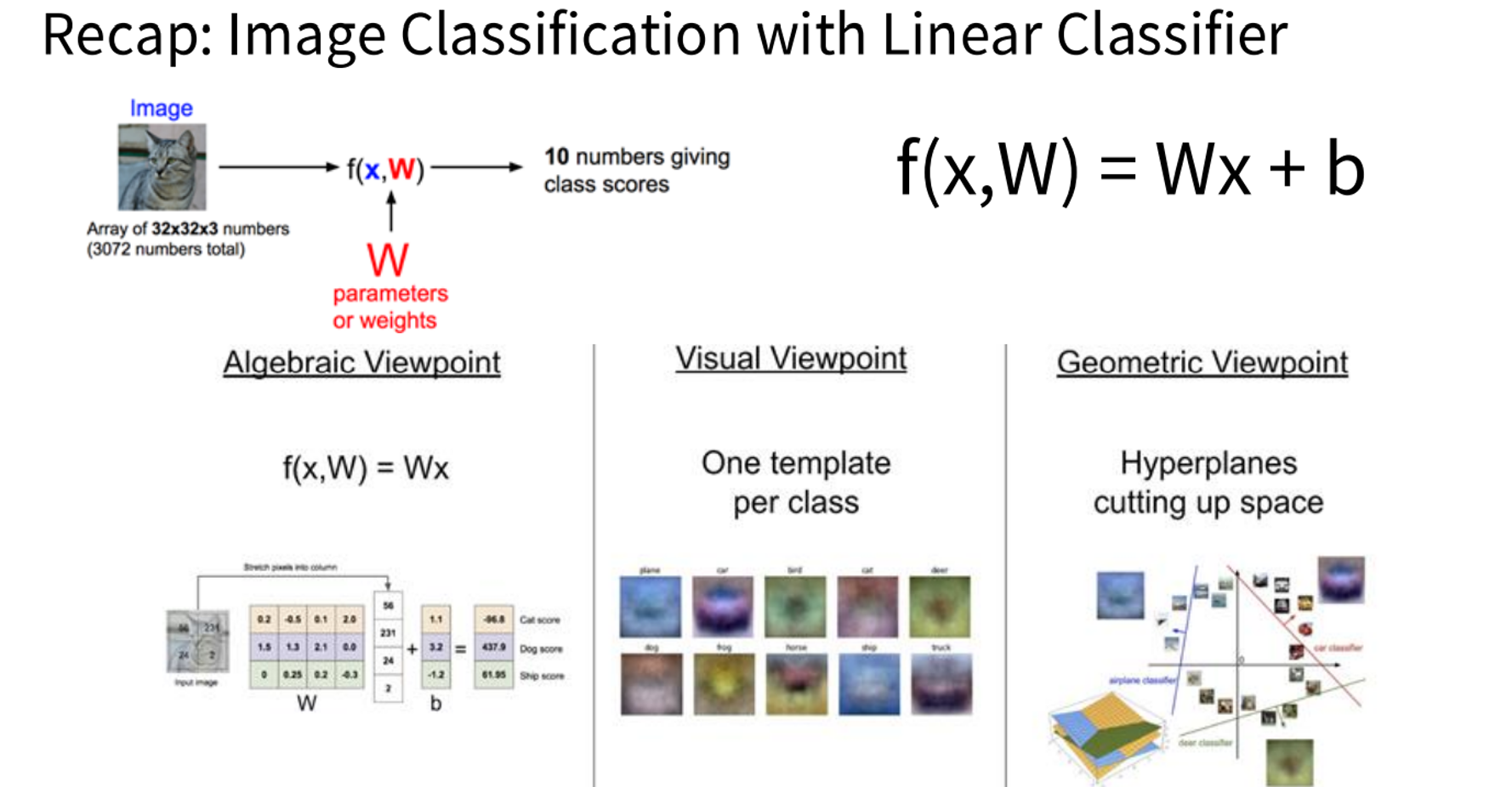
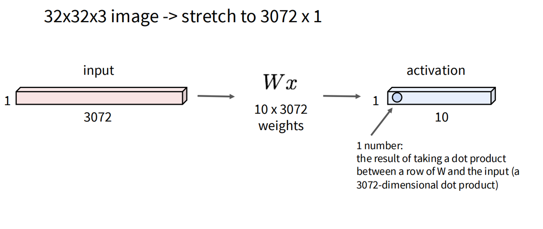
Traditionally, image classification can be approached using linear classifiers. In this approach, an image is represented as a high-dimensional vector, and a linear function $f(x,W) = Wx + b$ is used to compute class scores. Here, $x$ is the input image vector, $W$ represents the weights or parameters, and $b$ is the bias. For example, a 32x32x3 (width, height, RGB channels) image results in a total of 3072 numbers.

However, linear classifiers have limitations:

• They learn only one template per class.
• They can only draw linear decision boundaries, which might not be sufficient for complex image variations.

Neural Networks for Image Classification

Neural networks overcome the limitations of linear classifiers by introducing non-linearity. A 2-layer neural network, for instance, can be represented as $f = W_2 \max(0, W_1x)$. This structure allows the network to learn more complex patterns and non-linear decision boundaries.

A major challenge with traditional neural networks for image classification is that they flatten the image into a 1D vector, which destroys the spatial structure of the image. This loss of spatial information can be detrimental for tasks where the arrangement of pixels is crucial, such as recognizing objects in an image.

Convolutional Neural Networks (CNNs)

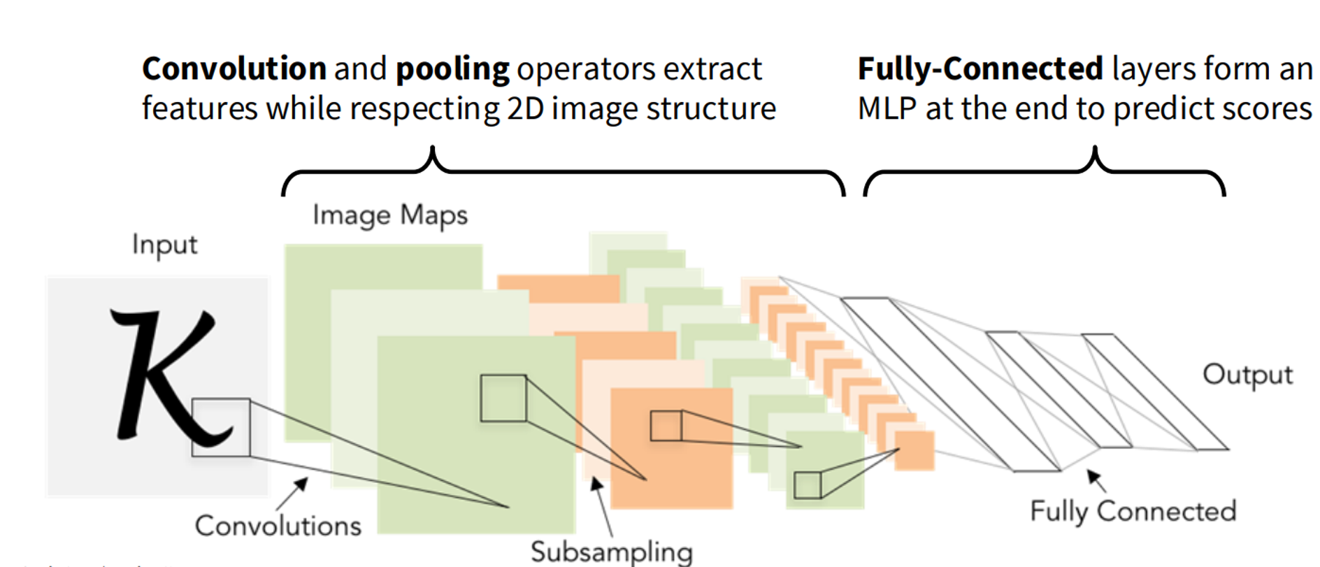
Convolutional Neural Networks (CNNs) are a special type of neural network designed to process data that has a known grid-like topology, like images. They address the limitations of traditional neural networks by preserving the spatial structure of images.

In a nutshell, CNNs employ two main types of layers:

1. Convolution and Pooling layers: These layers extract features while respecting the 2D image structure.
2. Fully-Connected layers: These layers, typically at the end of the network, form a Multi-Layer Perceptron (MLP) to predict scores for different classes.

Convolutional Layer Explained

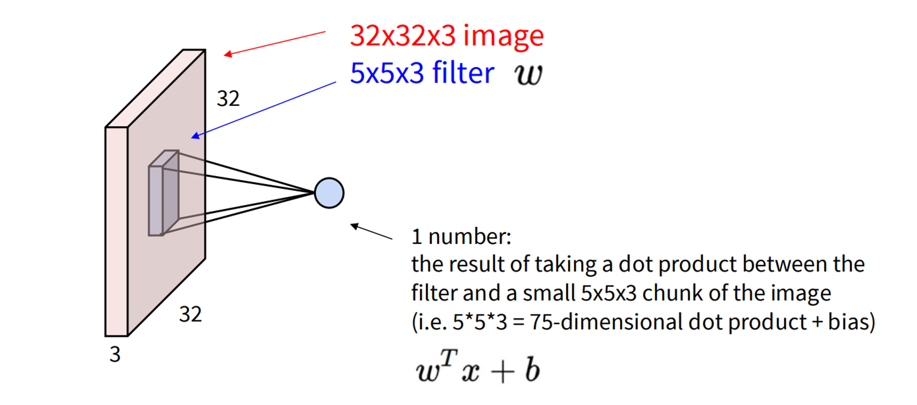
Unlike a linear layer that flattens a 32x32x3 image into a 3072x1 vector, a convolutional layer preserves the 32x32x3 spatial structure.

A key component of a convolutional layer is the filter (also known as a kernel). A filter is a small-dimensional array of numbers, for example, 5x5x3. The filter is convolved with the image by “sliding” it spatially over the image and computing a dot product between the filter and a small chunk of the image. This operation effectively extracts local features from the image. The filters always extend to the full depth of the input volume.

The output of convolving a single filter across the image is a 2D activation map. For a 32x32x3 image and a 5x5x3 filter, the activation map would be 28x28. If you use multiple filters (e.g., 6 filters), you get multiple activation maps (e.g., 6 activation maps, each 1x28x28), which are then stacked to form an output image. Along with filters, a bias vector is also added to the output.

For an input batch of images with dimensions $N \times C_{in} \times H \times W$, a convolutional layer with $C_{out}$ filters, each of size $C_{in} \times K_H \times K_W$, and a $C_{out}$-dimensional bias vector, produces an output batch of dimensions $N \times C_{out} \times H' \times W'$.

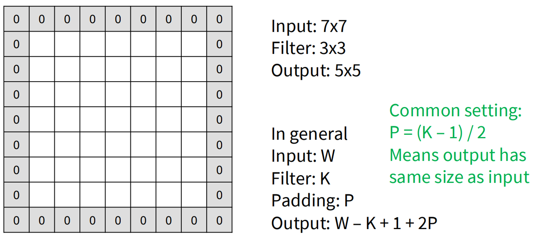
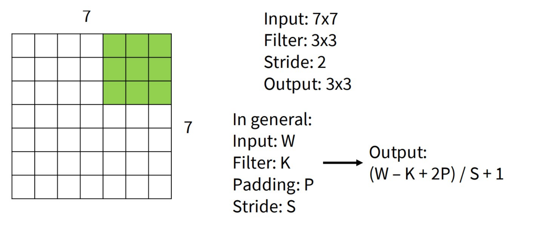
The output size of a convolutional layer is determined by the following formulas: $H' = (H - K_H + 2P) / S + 1$ $W' = (W - K_W + 2P) / S + 1$ where:

• $H, W$: Input height and width
• $K_H, K_W$: Kernel height and width
• $P$: Padding
• $S$: Stride

Padding is used to prevent feature maps from shrinking with each layer. By adding zeros around the input image, the output size can be maintained. A common setting for padding is $P = (K - 1) / 2$, which ensures the output has the same size as the input.

Stride refers to how many pixels the filter shifts at each step. A larger stride results in a smaller output volume, effectively downsampling the image.

Learnable Parameters and FLOPs in a Convolutional Layer

Consider an input volume of 3x32x32 and 10 5x5 filters with a stride of 1 and padding of 2. The number of learnable parameters for each filter is $3 \times 5 \times 5 + 1$ (for bias) = 76. With 10 filters, the total number of learnable parameters is $10 \times 76 = 760$.

The number of multiply-add operations (FLOPs) can be calculated as follows: Each output is the inner product of two 3x5x5 tensors (75 elements). The output volume size is 10x32x32 = 10,240 outputs. Total FLOPs = 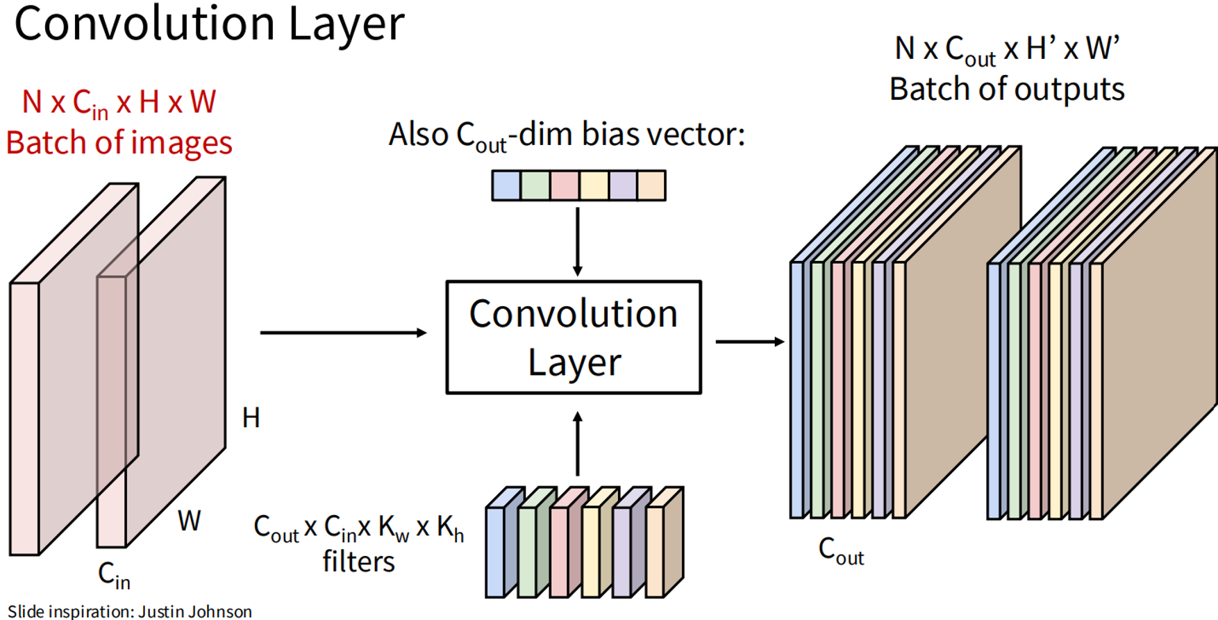$75 \times 10,240 = 768,000$.

Receptive Field

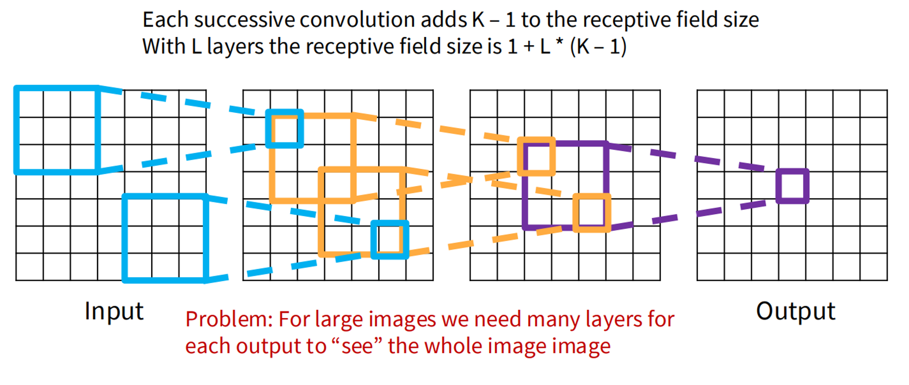
The receptive field refers to the region in the input that contributes to a particular element in the output. For a convolution with a kernel size $K$, each element in the output depends on a $K \times K$ receptive field in the input. As more convolutional layers are stacked, the receptive field grows. For $L$ layers, the receptive field size is $1 + L \times (K-1)$. However, for large images, many layers would be needed for each output to “see” the whole image, which is inefficient. The solution to this problem is to downsample inside the network, often using strided convolutions or pooling layers.

Pooling Layers

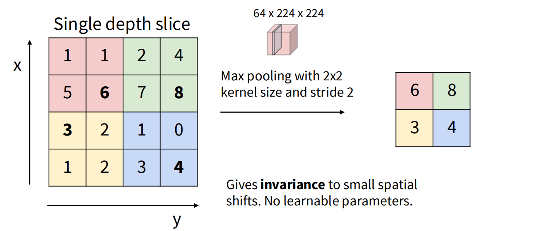
Pooling layers are another way to downsample the spatial dimensions of the input volume. They operate on each 1xHxW plane independently. Common pooling functions include max pooling and average pooling. For example, max pooling with a 2x2 kernel size and stride 2 will reduce the spatial dimensions by half. Pooling layers typically have no learnable parameters. Pooling layers provide a degree of translation invariance, meaning that features of images don’t depend on their exact location in the image.

What do CNN Filters Learn?

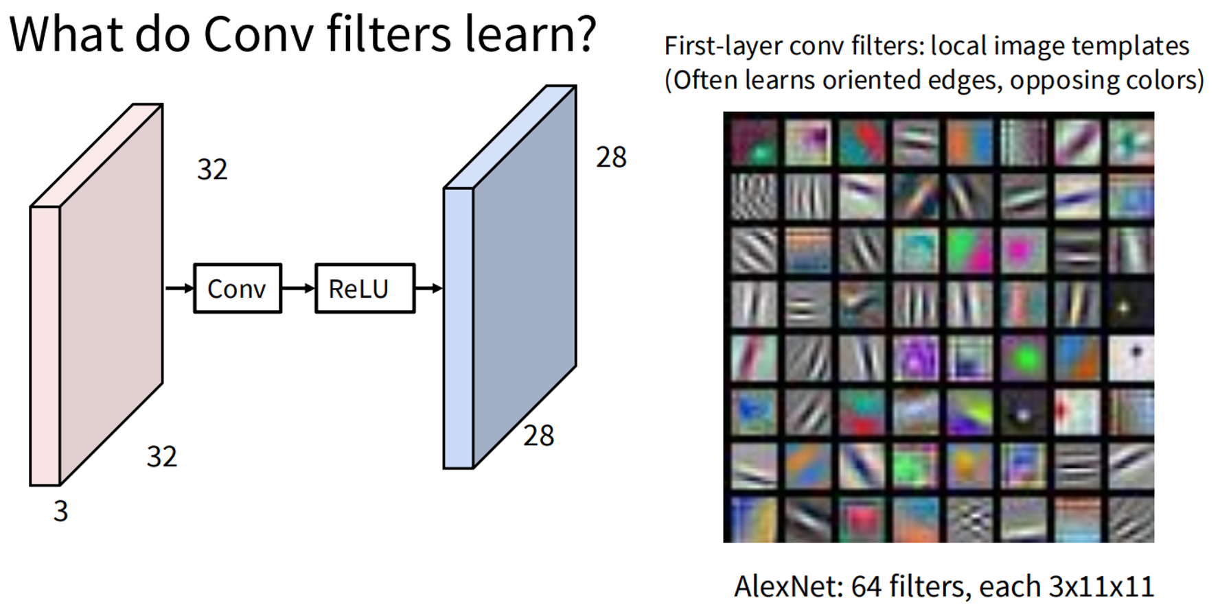
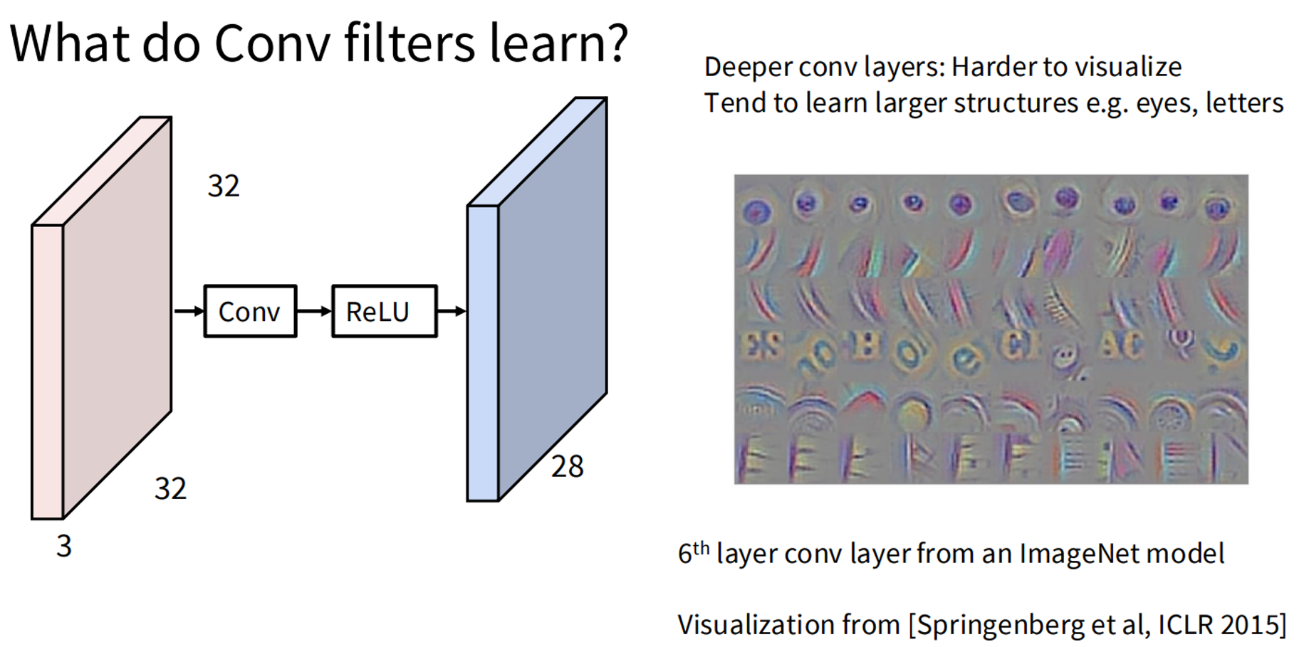
Early layers in a CNN often learn basic, local image templates like oriented edges and opposing colors. As the network gets deeper, the filters in deeper convolutional layers tend to learn larger and more complex structures, such as eyes or letters, which are harder to visualize directly.

PyTorch Implementation of a CNN (CIFAR-10 Demo)

Let’s build a simple CNN for the CIFAR-10 dataset using PyTorch. The CIFAR-10 dataset consists of 60,000 32x32 color images in 10 classes, with 6,000 images per class.

First, we need to import the necessary libraries.

import torch
import torch.nn as nn
import torch.optim as optim
import torchvision
import torchvision.transforms as transforms
import matplotlib.pyplot as plt
import numpy as np

1. Data Preparation

We’ll load the CIFAR-10 dataset and apply some basic transformations.

transform = transforms.Compose(
    [transforms.ToTensor(),
     transforms.Normalize((0.5, 0.5, 0.5), (0.5, 0.5, 0.5))])

trainset = torchvision.datasets.CIFAR10(root='./data', train=True,
                                        download=True, transform=transform)
trainloader = torch.utils.data.DataLoader(trainset, batch_size=4,
                                          shuffle=True, num_workers=2)

testset = torchvision.datasets.CIFAR10(root='./data', train=False,
                                       download=True, transform=transform)
testloader = torch.utils.data.DataLoader(testset, batch_size=4,
                                         shuffle=False, num_workers=2)

classes = ('plane', 'car', 'bird', 'cat',
           'deer', 'dog', 'frog', 'horse', 'ship', 'truck')

2. Define the CNN Architecture

We’ll create a simple CNN with two convolutional layers followed by max-pooling, and then three fully connected layers.

class Cifar10CnnModel(nn.Module):
    def __init__(self):
        super().__init__()
        self.network = nn.Sequential(
            nn.Conv2d(3, 32, kernel_size=3, padding=1),
            nn.ReLU(),
            nn.Conv2d(32, 64, kernel_size=3, stride=1, padding=1),
            nn.ReLU(),
            nn.MaxPool2d(2, 2), # output: 64 x 16 x 16

            nn.Conv2d(64, 128, kernel_size=3, stride=1, padding=1),
            nn.ReLU(),
            nn.Conv2d(128, 128, kernel_size=3, stride=1, padding=1),
            nn.ReLU(),
            nn.MaxPool2d(2, 2), # output: 128 x 8 x 8

            nn.Conv2d(128, 256, kernel_size=3, stride=1, padding=1),
            nn.ReLU(),
            nn.Conv2d(256, 256, kernel_size=3, stride=1, padding=1),
            nn.ReLU(),
            nn.MaxPool2d(2, 2), # output: 256 x 4 x 4

            nn.Flatten(), 
            nn.Linear(256*4*4, 1024),
            nn.ReLU(),
            nn.Linear(1024, 512),
            nn.ReLU(),
            nn.Linear(512, 10))
        
    def forward(self, xb):
        return self.network(xb)
model = Cifar10CnnModel().to(device)

3. Loss Function and Optimizer

We’ll use Cross-Entropy Loss and Stochastic Gradient Descent (SGD) for optimization.

criterion = nn.CrossEntropyLoss()
optimizer = optim.SGD(model.parameters(), lr=0.001, momentum=0.9)

4. Training the Network

print("Starting training...")
for epoch in range(5):  # loop over the dataset multiple times

    running_loss = 0.0
    for i, data in enumerate(trainloader, 0):
        inputs, labels = data

        optimizer.zero_grad() # zero the parameter gradients

        outputs = model(inputs)
        loss = criterion(outputs, labels)
        loss.backward()
        optimizer.step()

        running_loss += loss.item()
        if i % 2000 == 1999:    # print every 2000 mini-batches
            print(f'[{epoch + 1}, {i + 1:5d}] loss: {running_loss / 2000:.3f}')
            running_loss = 0.0

print("Finished training.")

# Save the trained model
PATH = './cifar_net.pth'
torch.save(model.state_dict(), PATH)

5. Testing the Network

# Load the trained model
model = SimpleCNN()
model.load_state_dict(torch.load(PATH))

correct = 0
total = 0
# since we're not training, we don't need to calculate the gradients for our outputs
with torch.no_grad():
    for data in testloader:
        images, labels = data
        # calculate outputs by running images through the network
        outputs = model(images)
        # the class with the highest energy is what we choose as prediction
        _, predicted = torch.max(outputs.data, 1)
        total += labels.size(0)
        correct += (predicted == labels).sum().item()

print(f'Accuracy of the network on the 10000 test images: {100 * correct // total} %')

# Per-class accuracy
class_correct = list(0. for i in range(10))
class_total = list(0. for i in range(10))
with torch.no_grad():
    for data in testloader:
        images, labels = data
        outputs = net(images)
        _, predicted = torch.max(outputs, 1)
        c = (predicted == labels).squeeze()
        for i in range(4):
            label = labels[i]
            class_correct[label] += c[i].item()
            class_total[label] += 1

print("\nAccuracy per class:")
for i in range(10):
    print(f'Accuracy of {classes[i]:5s} : {100 * class_correct[i] / class_total[i]:.2f} %')

6. Visualizing the Learned Filters

One of the fascinating aspects of CNNs is understanding what their filters learn. Let’s visualize the filters from the first convolutional layer (conv1) of our trained SimpleCNN.

# Function to visualize filters
def imshow_filters(filters, title="Learned Filters"):
    # Normalize filter values to [0, 1] for visualization
    filters_normalized = filters - filters.min()
    filters_normalized = filters_normalized / filters_normalized.max()

    num_filters = filters.shape[0]
    fig = plt.figure(figsize=(num_filters * 2, 2)) # Adjust figure size dynamically
    for i in range(num_filters):
        ax = fig.add_subplot(1, num_filters, i + 1)
        # Assuming filters are 3-channel for color images (like our conv1 filters)
        # Permute from (C_out, C_in, H, W) to (H, W, C_in) for imshow
        img = filters_normalized[i].cpu().numpy().transpose((1, 2, 0))
        ax.imshow(img)
        ax.axis('off')
    plt.suptitle(title)
    plt.show()

# Get the weights from the first convolutional layer
# Access the weights of the conv1 layer
conv1_weights = model.network[0].weight.data

print("Shape of conv1_weights:", conv1_weights.shape) # Expected: [6, 3, 5, 5] (out_channels, in_channels, H, W)

# Visualize the learned filters
imshow_filters(conv1_weights, "Learned Filters from conv1")

This code snippet will display the 6 filters learned by the first convolutional layer. Each filter is a 5x5x3 array. You might observe that these filters often represent basic visual features like edges or color gradients, which the network uses as building blocks to recognize more complex patterns in subsequent layers.

This concludes our blog post tutorial on Convolutional Neural Networks, covering their core concepts, their advantages for image classification, and a practical PyTorch implementation with filter visualization.