Transfer Learning with CNNs and Vision Transformers
Published on Thursday, 03-07-2025
Transfer Learning with CNNs and Vision Transformers: A Complete Guide
Understanding how to leverage pretrained models for better performance on your own datasets
Introduction
Transfer learning has revolutionized the field of computer vision by allowing us to leverage knowledge from large, pretrained models and apply it to smaller, specific datasets. In this comprehensive tutorial, we’ll explore transfer learning using two powerful architectures: Convolutional Neural Networks (CNNs) and Vision Transformers (ViTs).
Whether you’re working with limited data or want to achieve better performance faster, transfer learning is your go-to technique. Let’s dive deep into how it works and implement it step by step.
What is Transfer Learning?
Transfer learning is a machine learning technique where a model trained on one task is adapted for a related task. Think of it like this: if you’ve learned to play the piano, you’ll find it easier to learn the organ because you already understand musical concepts, reading sheet music, and finger coordination.
In computer vision, this means:
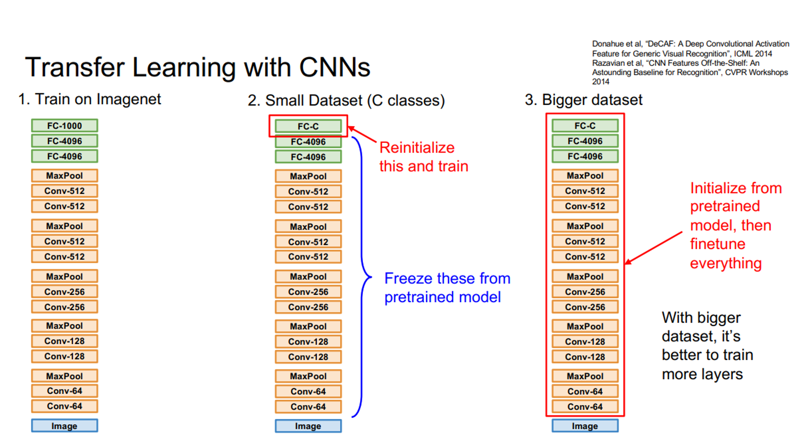
- Training on a large dataset (like ImageNet with 1.2 million images) to learn general visual features
- Fine-tuning on your smaller, specific dataset to adapt to your particular task
Why Transfer Learning Works
- Feature Reusability: Early layers learn universal features (edges, textures, shapes) that are useful across many tasks
- Data Efficiency: You don’t need massive datasets to achieve good performance
- Faster Training: Starting from pretrained weights converges much faster than training from scratch
- Better Performance: Often achieves higher accuracy than training from scratch
Understanding the Two Architectures
1. Convolutional Neural Networks (CNNs)
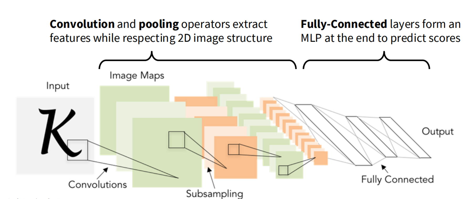
CNNs are the traditional workhorses of computer vision. They process images through:
- Convolutional layers: Extract local features using sliding filters
- Pooling layers: Reduce spatial dimensions while preserving important features
- Fully connected layers: Make final predictions
Key CNN Concepts:
- Local Receptive Fields: Each neuron only looks at a small region of the input
- Parameter Sharing: The same filter is applied across the entire image
- Hierarchical Feature Learning: Early layers learn simple features (edges), later layers learn complex features (objects)
ResNet Architecture: We’ll use ResNet-50, which introduced residual connections (skip connections) that allow gradients to flow more easily through very deep networks. This solved the vanishing gradient problem that plagued earlier deep CNNs.
2. Vision Transformers (ViTs)
ViTs are the newer kids on the block, applying the transformer architecture (originally designed for natural language processing) to computer vision.
How ViTs Work:
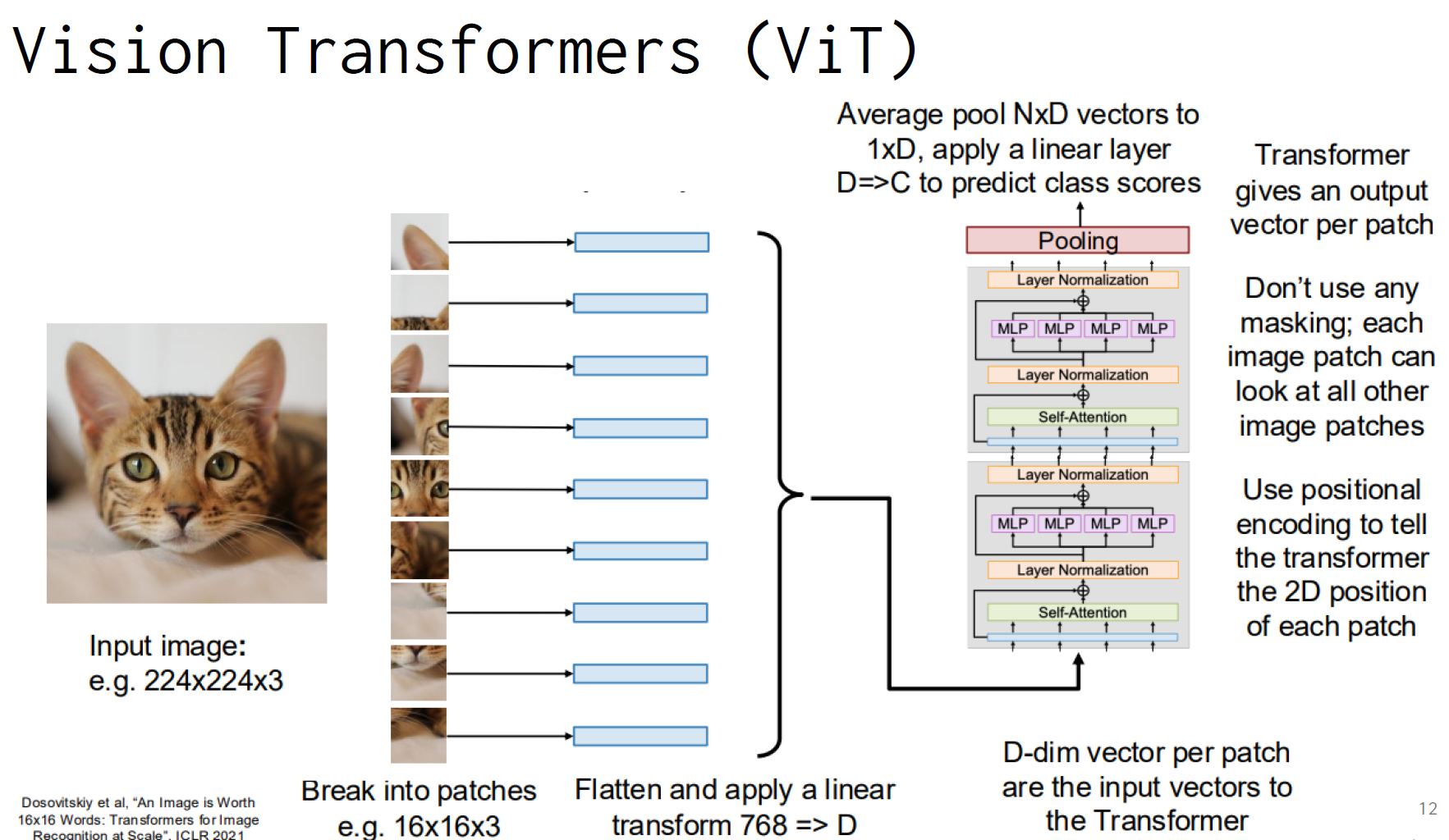
- Image Patching: Break the image into fixed-size patches (e.g., 16×16 pixels)
- Linear Projection: Flatten each patch and project it to a vector
- Positional Encoding: Add position information to maintain spatial relationships
- Transformer Blocks: Process patches through self-attention and feed-forward layers
- Classification Head: Average pool and classify
Key ViT Concepts:
- Global Attention: Each patch can attend to all other patches
- No Convolutions: Pure attention-based architecture
- Scalability: Can handle variable input sizes more easily than CNNs
Setting Up the Environment
Before we dive into the code, let’s set up our environment:
import torch
import torch.nn as nn
import torch.optim as optim
import torchvision
import torchvision.transforms as transforms
from transformers import ViTForImageClassification, ViTFeatureExtractor
import numpy as np
from sklearn.metrics import accuracy_score, precision_recall_fscore_support

# Set random seed for reproducibility
torch.manual_seed(42)
device = torch.device('cuda' if torch.cuda.is_available() else 'cpu')
Data Preprocessing: The Foundation of Success
Proper data preprocessing is crucial for transfer learning success. Let’s understand why each step matters:
CNN Data Transforms
# Training transforms with augmentation
cnn_transform_train = transforms.Compose([
    transforms.RandomHorizontalFlip(),  # Flip images horizontally
    transforms.RandomCrop(32, padding=4),  # Random crop with padding
    transforms.ToTensor(),  # Convert to tensor
    transforms.Normalize(mean=[0.4914, 0.4822, 0.4465],
                        std=[0.2023, 0.1994, 0.2010])  # Normalize
])

# Test transforms (no augmentation)
cnn_transform_test = transforms.Compose([
    transforms.ToTensor(),
    transforms.Normalize(mean=[0.4914, 0.4822, 0.4465],
                        std=[0.2023, 0.1994, 0.2010])
])
Why These Transforms Matter:
- RandomHorizontalFlip: Helps the model learn that objects can appear on either side
- RandomCrop: Teaches the model to be robust to slight position changes
- Normalization: Ensures all pixel values are in a similar range, helping with training stability
- No augmentation on test set: We want consistent evaluation
ViT Data Transforms
ViTs require specific preprocessing because they were trained on ImageNet with particular image sizes and normalization:
# ViT feature extractor handles the preprocessing
vit_feature_extractor = ViTFeatureExtractor.from_pretrained('google/vit-base-patch16-224-in21k')

# Custom dataset class for ViT
class CIFAR10ForViT(torch.utils.data.Dataset):
    def __init__(self, root, train, feature_extractor):
        self.dataset = torchvision.datasets.CIFAR10(root=root, train=train, download=True)
        self.feature_extractor = feature_extractor

    def __len__(self):
        return len(self.dataset)

    def __getitem__(self, idx):
        image, label = self.dataset[idx]
        inputs = self.feature_extractor(images=image, return_tensors='pt')
        return inputs['pixel_values'].squeeze(0), label
Loading and Modifying Pretrained Models
Loading ResNet-50
# Load pretrained ResNet-50
resnet = torchvision.models.resnet50(pretrained=True)

# Modify the final layer for our task
resnet.fc = nn.Linear(resnet.fc.in_features, 10)  # 10 classes for CIFAR-10
resnet = resnet.to(device)
What’s Happening Here:
- We load ResNet-50 pretrained on ImageNet (1000 classes)
- We replace the final fully connected layer to output 10 classes (CIFAR-10)
- The pretrained weights in the convolutional layers remain unchanged
Loading Vision Transformer
# Load pretrained ViT
vit = ViTForImageClassification.from_pretrained(
    'google/vit-base-patch16-224-in21k',
    num_labels=10
)
vit = vit.to(device)
Key Differences:
- ViT automatically adjusts the classifier head for our number of classes
- The transformer blocks remain pretrained
- Positional encodings are preserved
Understanding the Fine-Tuning Process
Fine-tuning is where the magic happens. We need to be careful not to destroy the valuable pretrained features while adapting to our new task.
Learning Rate Selection
# Different learning rates for different architectures
optimizer_resnet = optim.SGD(resnet.parameters(), lr=1e-3, momentum=0.9, weight_decay=1e-4)
optimizer_vit = optim.AdamW(vit.parameters(), lr=1e-5, weight_decay=1e-4)
Why Different Learning Rates:
- ResNet: Higher learning rate (1e-3) because CNNs are more robust to learning rate changes
- ViT: Lower learning rate (1e-5) because transformers are more sensitive to learning rate changes
- Weight Decay: Prevents overfitting by penalizing large weights
Training Function
def train_model(model, train_loader, optimizer, criterion, epochs=3, is_vit=False):
    model.train()
    for epoch in range(epochs):
        running_loss = 0.0
        for inputs, labels in train_loader:
            inputs, labels = inputs.to(device), labels.to(device)

            optimizer.zero_grad()  # Clear previous gradients

            # Forward pass
            if is_vit:
                outputs = model(inputs).logits  # ViT returns a dict
            else:
                outputs = model(inputs)  # CNN returns logits directly

            # Compute loss
            loss = criterion(outputs, labels)

            # Backward pass
            loss.backward()
            optimizer.step()

            running_loss += loss.item()

        print(f'Epoch {epoch+1}, Loss: {running_loss/len(train_loader):.4f}')
Key Training Concepts:
- Model.train(): Enables training mode (enables dropout, batch norm updates)
- optimizer.zero_grad(): Clears gradients from previous batch
- Loss.backward(): Computes gradients
- optimizer.step(): Updates model parameters
Evaluation: Measuring Success
Evaluation is crucial to understand how well our models generalize to unseen data.
def evaluate_model(model, test_loader, criterion, is_vit=False):
    model.eval()  # Set to evaluation mode
    test_loss = 0.0
    all_preds = []
    all_labels = []

    with torch.no_grad():  # Disable gradient computation
        for inputs, labels in test_loader:
            inputs, labels = inputs.to(device), labels.to(device)

            # Forward pass
            if is_vit:
                outputs = model(inputs).logits
            else:
                outputs = model(inputs)

            # Compute loss
            loss = criterion(outputs, labels)
            test_loss += loss.item()

            # Get predictions
            _, preds = torch.max(outputs, 1)
            all_preds.extend(preds.cpu().numpy())
            all_labels.extend(labels.cpu().numpy())

    # Compute metrics
    accuracy = accuracy_score(all_labels, all_preds)
    precision, recall, f1, _ = precision_recall_fscore_support(
        all_labels, all_preds, average='weighted'
    )
    avg_loss = test_loss / len(test_loader)

    print(f'Test Loss: {avg_loss:.4f}')
    print(f'Accuracy: {accuracy:.4f}')
    print(f'Precision: {precision:.4f}')
    print(f'Recall: {recall:.4f}')
    print(f'F1-Score: {f1:.4f}')
Evaluation Metrics Explained:
- Accuracy: Percentage of correct predictions
- Precision: Of the predictions we made, how many were correct?
- Recall: Of the actual positives, how many did we catch?
- F1-Score: Harmonic mean of precision and recall (balanced metric)
Key Differences Between CNN and ViT Transfer Learning
1. Input Processing
CNN:
- Processes images directly through convolutional layers
- Maintains spatial structure throughout the network
- Uses local receptive fields
ViT:
- Breaks images into patches first
- Processes patches as a sequence
- Uses global attention mechanisms
2. Training Dynamics
CNN:
- More stable training
- Can handle higher learning rates
- Benefits from data augmentation
ViT:
- More sensitive to hyperparameters
- Requires careful learning rate tuning
- May need more data to perform well
3. Computational Requirements
CNN:
- Generally faster to train
- Lower memory requirements
- Well-optimized on GPUs
ViT:
- Can be slower due to attention computations
- Higher memory requirements
- Benefits from larger batch sizes
Best Practices for Transfer Learning
1. Learning Rate Scheduling
# Example of learning rate scheduling
scheduler = optim.lr_scheduler.StepLR(optimizer, step_size=30, gamma=0.1)
2. Gradual Unfreezing
# Freeze early layers, train later layers first
for param in model.layer1.parameters():
    param.requires_grad = False

# Train for a few epochs
# Then unfreeze and train with lower learning rate
for param in model.parameters():
    param.requires_grad = True
3. Data Augmentation Strategies
# More aggressive augmentation for smaller datasets
transforms.Compose([
    transforms.RandomHorizontalFlip(),
    transforms.RandomRotation(10),
    transforms.ColorJitter(brightness=0.2, contrast=0.2),
    transforms.RandomResizedCrop(224, scale=(0.8, 1.0)),
    transforms.ToTensor(),
    transforms.Normalize(mean, std)
])
Common Pitfalls and How to Avoid Them
1. Learning Rate Too High
Problem: Destroys pretrained features Solution: Start with low learning rates (1e-4 to 1e-5)
2. Insufficient Data Augmentation
Problem: Model overfits to training data Solution: Use appropriate augmentation for your dataset size
3. Wrong Normalization
Problem: Model performs poorly due to distribution mismatch Solution: Use the same normalization as the pretrained model
4. Not Monitoring Validation Loss
Problem: Overfitting goes unnoticed Solution: Always use a validation set and early stopping
Advanced Techniques
1. Knowledge Distillation
Train a smaller model to mimic a larger pretrained model:
# Teacher model (large, pretrained)
teacher_model = load_pretrained_model()

# Student model (smaller)
student_model = create_smaller_model()

# Distillation loss
def distillation_loss(student_output, teacher_output, temperature=4.0):
    return F.kl_div(
        F.log_softmax(student_output / temperature, dim=1),
        F.softmax(teacher_output / temperature, dim=1),
        reduction='batchmean'
    ) * (temperature ** 2)
2. Progressive Unfreezing
# Train in stages
# Stage 1: Only classifier
freeze_backbone(model)
train_epochs(model, epochs=5)

# Stage 2: Last few layers
unfreeze_layers(model, layers=['layer4'])
train_epochs(model, epochs=5)

# Stage 3: All layers
unfreeze_all(model)
train_epochs(model, epochs=10)
Conclusion
Transfer learning is a powerful technique that has democratized deep learning in computer vision. By leveraging pretrained models, you can achieve excellent results even with limited data and computational resources.
Key Takeaways:
- Choose the right architecture: CNNs for traditional computer vision tasks, ViTs for tasks requiring global context
- Preprocess data correctly: Use appropriate normalization and augmentation
- Fine-tune carefully: Use low learning rates and monitor validation performance
- Evaluate thoroughly: Use multiple metrics to understand model performance
- Iterate and experiment: Transfer learning is as much art as science
Whether you’re working on image classification, object detection, or any other computer vision task, transfer learning should be your first approach. The combination of pretrained knowledge and task-specific fine-tuning often leads to the best results.
Happy coding and happy learning! 🚀