(Adopted from https://introtodeeplearning.com/)

Deep Generative Modeling

Generative models are a fascinating subset of deep learning that focus on creating new data instances that resemble a given training dataset. Unlike discriminative models that classify or predict labels, generative models learn the underlying distribution of the data to produce novel samples. This has applications in image synthesis, data augmentation, debiasing datasets, and even simulating rare events for training robust systems like self-driving cars.

In this post, we’ll break down the key concepts step by step, starting from the basics of unsupervised learning and generative modeling, then diving into autoencoders, variational autoencoders (VAEs), and generative adversarial networks (GANs). We’ll explain each idea in detail, include mathematical formulations wrapped in LaTeX, and provide practical PyTorch code examples where applicable. By the end, you’ll have a solid understanding of how to implement these models yourself.

1. Introduction to Generative Modeling

Supervised vs. Unsupervised Learning

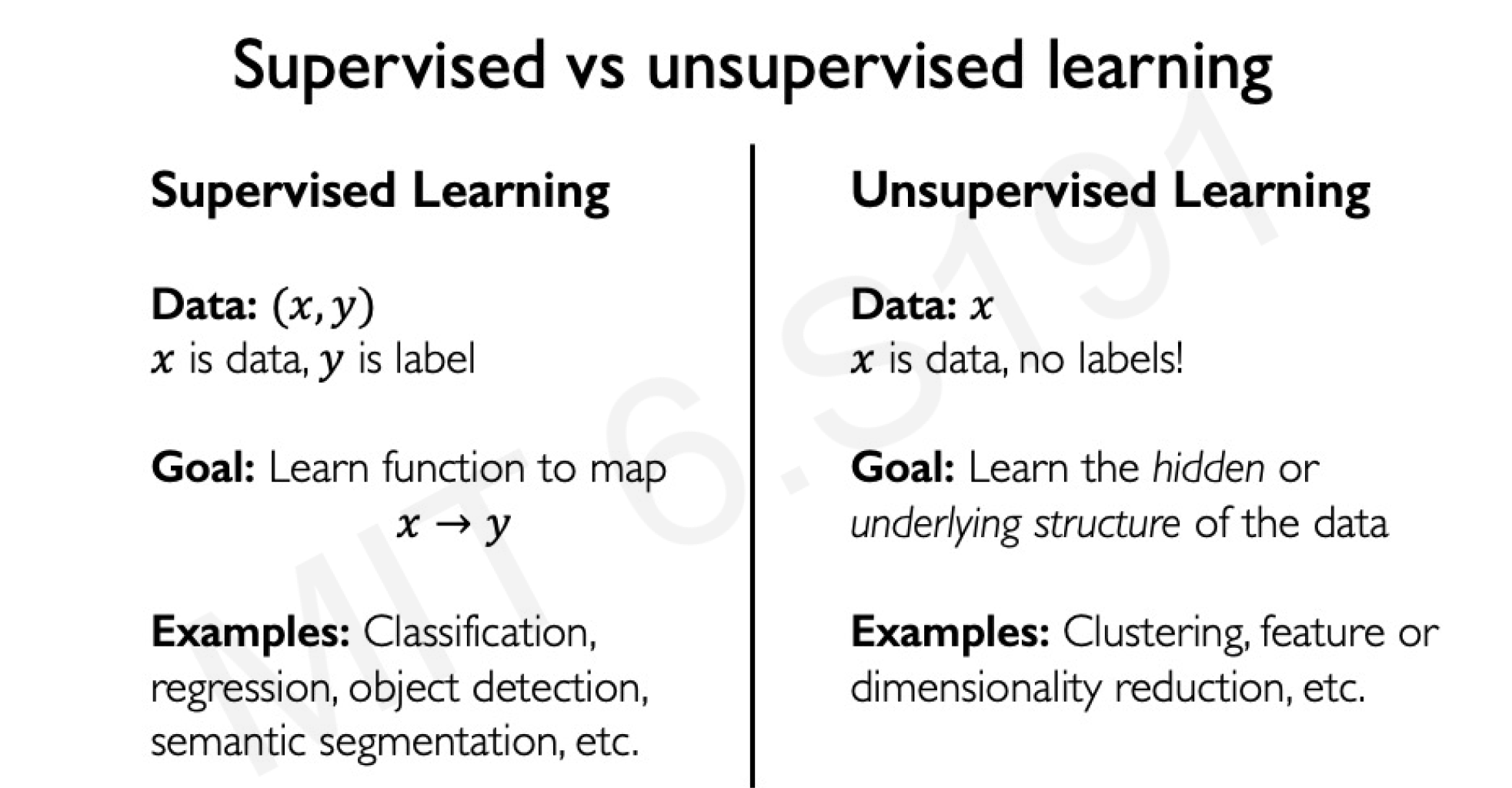
Deep learning models are broadly categorized into supervised and unsupervised learning paradigms.

• Supervised Learning: Models learn a mapping from input data $x$ to labels $y$, e.g., classifying images as cats or dogs. The goal is to approximate a function $f(x) \approx y$.

• Unsupervised Learning: Models are trained on data without labels, aiming to discover hidden patterns or structures. Examples include clustering (e.g., K-means) and dimensionality reduction (e.g., PCA).

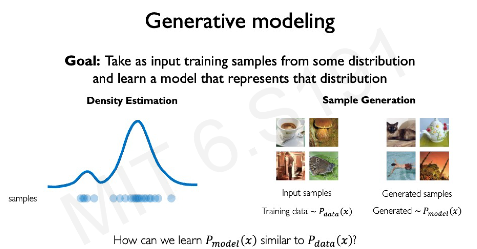
Generative modeling falls under unsupervised learning. The objective is to learn the probability distribution $p(x)$ of the training data so that new samples can be generated from it.

Goals of Generative Models

Given a dataset drawn from some unknown distribution $p_{\text{data}}(x)$, a generative model $G$ learns a distribution $p_G(x)$ that approximates $p_{\text{data}}(x)$. Once trained, $G$ can sample new data points $\hat{x} \sim p_G(x)$.

Why is this useful?

• Data Augmentation: Generate synthetic data to expand datasets, especially for underrepresented classes.
• Debiasing: Create balanced datasets by generating samples that counter biases (e.g., diverse facial images for fairer face recognition).
• Outlier Detection and Simulation: Model rare events (e.g., pedestrians jaywalking) for training safer AI systems.
• Creative Applications: Synthesize images, music, or text.

Generative models often use latent variables $z$, which capture hidden features in a lower-dimensional space. The model learns to map from $z$ (e.g., random noise) to $x$ (data).

2. Autoencoders: The Foundation of Representation Learning

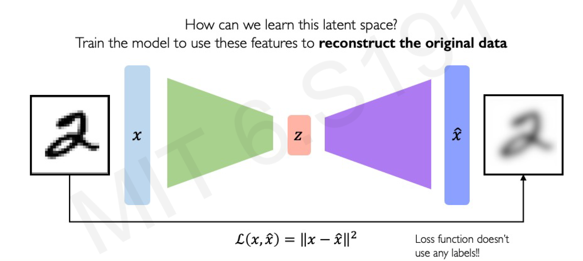
Autoencoders are neural networks that learn to compress and reconstruct data, serving as a building block for generative models. They consist of two parts: an encoder that maps input data to a latent space, and a decoder that reconstructs the input from the latent representation.

Key Concepts

• Encoder: $z = \text{Encoder}(x)$, where $z$ is a compact representation (bottleneck) in a lower-dimensional latent space.
• Decoder: $\hat{x} = \text{Decoder}(z)$, aiming to reconstruct $x$ as closely as possible.
• Training Objective: Minimize the reconstruction loss, typically Mean Squared Error (MSE) for continuous data like images:
  $$\mathcal{L} = \frac{1}{N} \sum_{i=1}^N \| x_i - \hat{x}_i \|^2$$
  This encourages the model to learn meaningful features in $z$ without labels.

Autoencoders are useful for dimensionality reduction, denoising, and as a precursor to more advanced generative models. However, standard autoencoders are deterministic and don’t explicitly model probabilities, limiting their generative capabilities.

PyTorch Implementation: Simple Autoencoder for MNIST

Let’s implement a basic autoencoder using PyTorch on the MNIST dataset (handwritten digits). We’ll use fully connected layers for simplicity.

import torch
import torch.nn as nn
import torch.optim as optim
from torchvision import datasets, transforms
from torch.utils.data import DataLoader

# Device configuration
device = torch.device('cuda' if torch.cuda.is_available() else 'cpu')

# Hyperparameters
latent_dim = 64
batch_size = 128
epochs = 10
learning_rate = 1e-3

# Data loader
transform = transforms.Compose([transforms.ToTensor()])
train_dataset = datasets.MNIST(root='./data', train=True, transform=transform, download=True)
train_loader = DataLoader(train_dataset, batch_size=batch_size, shuffle=True)

# Autoencoder model
class Autoencoder(nn.Module):
    def __init__(self):
        super(Autoencoder, self).__init__()
        self.encoder = nn.Sequential(
            nn.Linear(28*28, 128),
            nn.ReLU(),
            nn.Linear(128, latent_dim)
        )
        self.decoder = nn.Sequential(
            nn.Linear(latent_dim, 128),
            nn.ReLU(),
            nn.Linear(128, 28*28),
            nn.Sigmoid()  # Output between 0 and 1
        )

    def forward(self, x):
        x = x.view(-1, 28*28)  # Flatten
        z = self.encoder(x)
        x_hat = self.decoder(z)
        return x_hat.view(-1, 1, 28, 28)  # Reshape back to image

# Initialize model, loss, optimizer
model = Autoencoder().to(device)
criterion = nn.MSELoss()
optimizer = optim.Adam(model.parameters(), lr=learning_rate)

# Training loop
for epoch in range(epochs):
    model.train()
    train_loss = 0
    for data, _ in train_loader:
        data = data.to(device)
        optimizer.zero_grad()
        output = model(data)
        loss = criterion(output, data)
        loss.backward()
        optimizer.step()
        train_loss += loss.item()
    print(f'Epoch [{epoch+1}/{epochs}], Loss: {train_loss / len(train_loader):.4f}')

# To generate/reconstruct: Pass input through model

This code trains the autoencoder to reconstruct MNIST images. To “generate” (though not truly novel), you can encode an image to $z$ and decode it. For better results, use convolutional layers for images.

3. Variational Autoencoders (VAEs): Probabilistic Generative Models

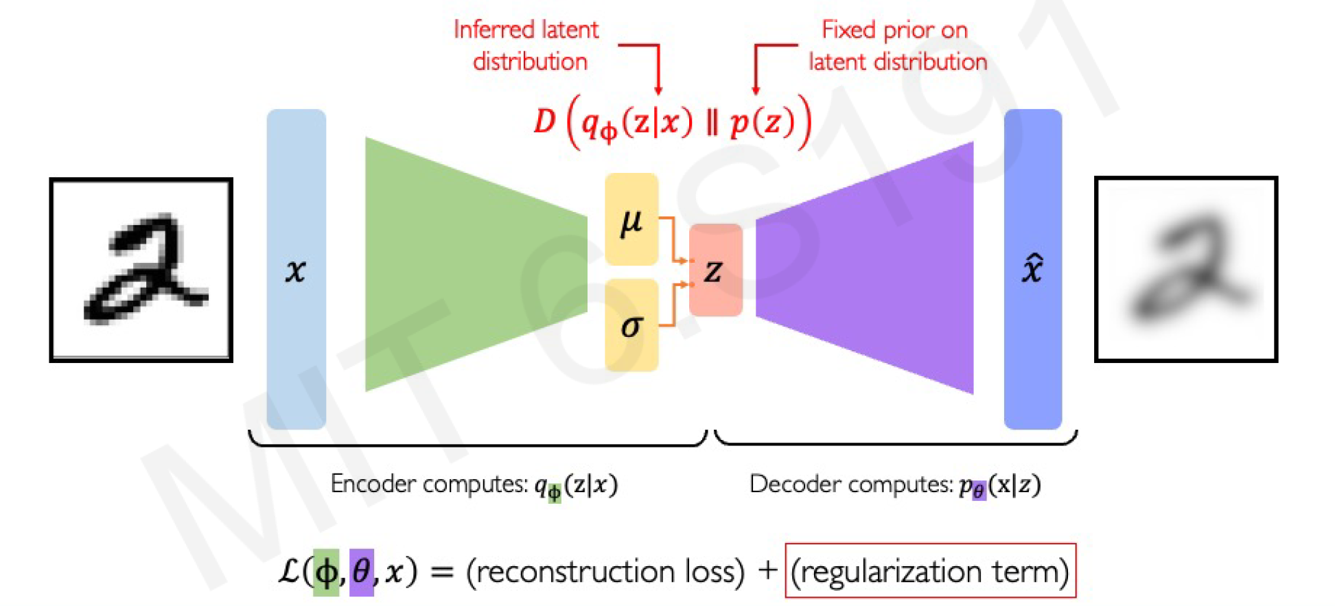
VAEs extend autoencoders by introducing probabilistic elements, making them true generative models. Instead of a fixed $z$, VAEs learn a distribution over the latent space, typically a Gaussian $q(z|x) \sim \mathcal{N}(\mu, \sigma^2)$.

Key Concepts

• Encoder: Outputs parameters of the latent distribution, e.g., mean $\mu$ and variance $\sigma^2$ (often log-variance for stability).
• Sampling: Draw $z$ from the distribution: $z = \mu + \sigma \odot \epsilon$, where $\epsilon \sim \mathcal{N}(0,1)$. This is the reparameterization trick, which allows backpropagation through the stochastic sampling.
• Decoder: Generates $\hat{x}$ from sampled $z$.
• Training Objective: Maximize the Evidence Lower Bound (ELBO):
  $$\mathcal{L}(\theta, \phi; x) = \mathbb{E}_{q_\phi(z|x)} [\log p_\theta(x|z)] - D_{KL}(q_\phi(z|x) \| p(z))$$
  • Reconstruction term: $\mathbb{E} [\log p(x|z)]$ (e.g., negative MSE or binary cross-entropy).
  • KL Divergence: Regularizes the latent distribution to match a prior $p(z) = \mathcal{N}(0,1)$, preventing overfitting. The full loss is the negative ELBO, minimized during training.

VAEs enable smooth interpolation in latent space and generation by sampling $z$ from the prior.

PyTorch Implementation: VAE for MNIST

We’ll modify the autoencoder to output $\mu$ and $\log \sigma^2$, add sampling, and compute the ELBO loss.

class VAE(nn.Module):
    def __init__(self):
        super(VAE, self).__init__()
        self.encoder_fc1 = nn.Linear(28*28, 128)
        self.encoder_mu = nn.Linear(128, latent_dim)
        self.encoder_logvar = nn.Linear(128, latent_dim)
        self.decoder_fc1 = nn.Linear(latent_dim, 128)
        self.decoder_fc2 = nn.Linear(128, 28*28)

    def encode(self, x):
        x = x.view(-1, 28*28)
        h = torch.relu(self.encoder_fc1(x))
        return self.encoder_mu(h), self.encoder_logvar(h)

    def reparameterize(self, mu, logvar):
        std = torch.exp(0.5 * logvar)
        eps = torch.randn_like(std)
        return mu + eps * std

    def decode(self, z):
        h = torch.relu(self.decoder_fc1(z))
        return torch.sigmoid(self.decoder_fc2(h)).view(-1, 1, 28, 28)

    def forward(self, x):
        mu, logvar = self.encode(x)
        z = self.reparameterize(mu, logvar)
        return self.decode(z), mu, logvar

# VAE Loss function
def vae_loss(recon_x, x, mu, logvar):
    BCE = nn.functional.binary_cross_entropy(recon_x.view(-1, 784), x.view(-1, 784), reduction='sum')
    KLD = -0.5 * torch.sum(1 + logvar - mu.pow(2) - logvar.exp())
    return (BCE + KLD) / x.size(0)  # Normalize by batch size

# Training (similar to autoencoder, but use vae_loss)
model = VAE().to(device)
optimizer = optim.Adam(model.parameters(), lr=learning_rate)

for epoch in range(epochs):
    model.train()
    train_loss = 0
    for data, _ in train_loader:
        data = data.to(device)
        optimizer.zero_grad()
        recon_batch, mu, logvar = model(data)
        loss = vae_loss(recon_batch, data, mu, logvar)
        loss.backward()
        optimizer.step()
        train_loss += loss.item()
    print(f'Epoch [{epoch+1}/{epochs}], Loss: {train_loss / len(train_loader):.4f}')

# To generate: Sample z from N(0,1) and decode
with torch.no_grad():
    z = torch.randn(64, latent_dim).to(device)
    samples = model.decode(z)

This VAE can generate new digit images by sampling random $z$.

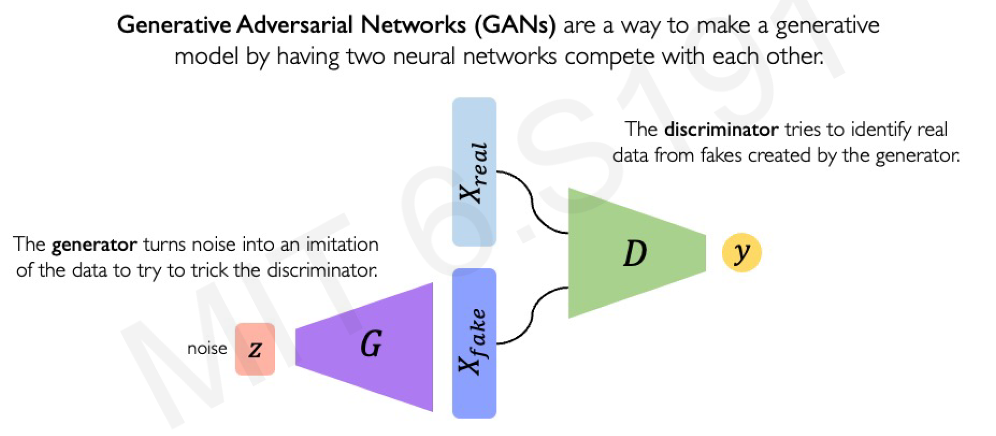
4. Generative Adversarial Networks (GANs): Adversarial Training

GANs introduce a game-theoretic approach with two networks: a Generator (G) that creates fake data from noise, and a Discriminator (D) that distinguishes real from fake data.

Key Concepts

• Generator: $G(z)$, maps latent noise $z \sim p_z(z)$ (e.g., $\mathcal{N}(0,1)$) to fake data $\hat{x}$.
• Discriminator: $D(x)$, outputs a probability that $x$ is real (1) or fake (0).
• Training Objective: Minimax game:
  $$\min_G \max_D V(D, G) = \mathbb{E}_{x \sim p_{\text{data}}} [\log D(x)] + \mathbb{E}_{z \sim p_z} [\log (1 - D(G(z)))]$$
  • D maximizes the value (learns to detect fakes).
  • G minimizes it (learns to fool D). Training alternates: Update D on real and fake batches, then update G based on D’s feedback.

GANs excel at high-quality image generation but can suffer from mode collapse (G produces limited variety) or instability.

PyTorch Implementation: Simple GAN for MNIST

We’ll use fully connected layers again.

class Generator(nn.Module):
    def __init__(self):
        super(Generator, self).__init__()
        self.model = nn.Sequential(
            nn.Linear(latent_dim, 128),
            nn.ReLU(),
            nn.Linear(128, 28*28),
            nn.Tanh()  # Output between -1 and 1 (normalize MNIST to -1/1)
        )

    def forward(self, z):
        return self.model(z).view(-1, 1, 28, 28)

class Discriminator(nn.Module):
    def __init__(self):
        super(Discriminator, self).__init__()
        self.model = nn.Sequential(
            nn.Linear(28*28, 128),
            nn.ReLU(),
            nn.Linear(128, 1),
            nn.Sigmoid()
        )

    def forward(self, x):
        return self.model(x.view(-1, 28*28))

# Initialize models
generator = Generator().to(device)
discriminator = Discriminator().to(device)
g_optimizer = optim.Adam(generator.parameters(), lr=learning_rate)
d_optimizer = optim.Adam(discriminator.parameters(), lr=learning_rate)
criterion = nn.BCELoss()

# Normalize MNIST to [-1, 1]
transform = transforms.Compose([transforms.ToTensor(), transforms.Normalize((0.5,), (0.5,))])
train_dataset = datasets.MNIST(root='./data', train=True, transform=transform, download=True)
train_loader = DataLoader(train_dataset, batch_size=batch_size, shuffle=True)

# Training loop
for epoch in range(epochs):
    for i, (images, _) in enumerate(train_loader):
        images = images.to(device)
        real_labels = torch.ones(images.size(0), 1).to(device)
        fake_labels = torch.zeros(images.size(0), 1).to(device)

        # Train Discriminator
        d_optimizer.zero_grad()
        real_outputs = discriminator(images)
        d_real_loss = criterion(real_outputs, real_labels)
        z = torch.randn(images.size(0), latent_dim).to(device)
        fake_images = generator(z)
        fake_outputs = discriminator(fake_images.detach())
        d_fake_loss = criterion(fake_outputs, fake_labels)
        d_loss = d_real_loss + d_fake_loss
        d_loss.backward()
        d_optimizer.step()

        # Train Generator
        g_optimizer.zero_grad()
        fake_outputs = discriminator(fake_images)
        g_loss = criterion(fake_outputs, real_labels)  # Fool D
        g_loss.backward()
        g_optimizer.step()

    print(f'Epoch [{epoch+1}/{epochs}], D Loss: {d_loss.item():.4f}, G Loss: {g_loss.item():.4f}')

# To generate: Sample z and pass through generator
with torch.no_grad():
    z = torch.randn(64, latent_dim).to(device)
    generated = generator(z)

This GAN learns to generate MNIST-like digits. For better quality, use DCGAN with convolutions.

Conclusion

Deep generative modeling opens up exciting possibilities for creating realistic data and understanding complex distributions. We covered autoencoders for representation learning, VAEs for probabilistic generation, and GANs for adversarial high-fidelity synthesis. Experiment with these PyTorch codes on datasets like CIFAR-10 for more challenges. For further reading, check the MIT course resources or explore advanced topics like diffusion models.

If you have questions or want to extend this to specific applications, drop a comment below!