Demystifying Image Classification - From Pixels to Predictions

(Adopted from CS231n - Computer Vision with Deep Learning)

Demystifying Image Classification: From Pixels to Predictions

Image classification is a fundamental task in computer vision, where the goal is to assign a label to an input image from a predefined set of categories. For example, given an image, we might want to classify it as a “cat,” “dog,” “truck,” or “plane”. While seemingly straightforward for humans, this task presents several challenges for computers.

The Challenges of Image Classification

Computers perceive images as grids of pixel values, typically integers between 0 and 255. Translating these raw pixel values into meaningful high-level concepts (like “cat”) is difficult due to several factors:

• Viewpoint Variation: An object can be viewed from different angles, causing significant changes in its pixel representation.
• Illumination Changes: Lighting conditions drastically alter pixel intensities, even for the same object.
• Background Clutter: The presence of distracting elements in the background can make it hard to isolate the object of interest.
• Occlusion: Parts of the object might be hidden from view, making identification challenging.
• Deformation: Objects can change shape or be in various poses.
• Intraclass Variation: Even within the same class (e.g., “cat”), there’s a wide variety of appearances.
• Context: Sometimes, the surrounding environment helps in identifying an object, but this context can also be misleading.

Viewpoints: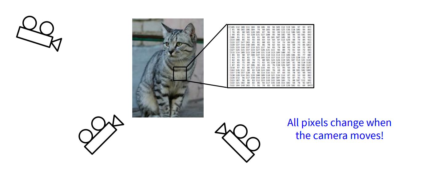

Illuminations: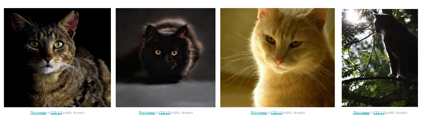

Given these complexities, directly hard-coding rules for classification is impractical. This leads us to a data-driven approach.

The Data-Driven Approach to Image Classification

Instead of defining explicit rules, machine learning relies on data to learn patterns. The process typically involves:

1. Collecting a dataset of images, each accompanied by its correct label.
2. Using machine learning algorithms to train a classifier on this dataset.
3. Evaluating the trained classifier on new, unseen images to assess its performance.

Let’s explore two foundational data-driven approaches: K-Nearest Neighbors and Linear Classifiers.

K-Nearest Neighbors (KNN)

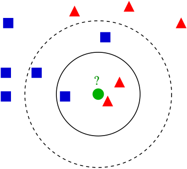
The K-Nearest Neighbors (KNN) algorithm is one of the simplest classification algorithms. Its core idea is that similar things exist in close proximity.

How KNN Works

• Training Phase: The KNN classifier simply “memorizes” all the training data and their corresponding labels. There’s no explicit model learning in this phase.
• Prediction Phase: To classify a new, unseen image, the KNN algorithm calculates its distance to every image in the training set. It then identifies the ‘K’ training images that are “nearest” (most similar) to the new image. The label for the new image is determined by a majority vote among these K nearest neighbors.

Distance Metrics

To measure similarity between images, we need a distance metric. Two common metrics are:

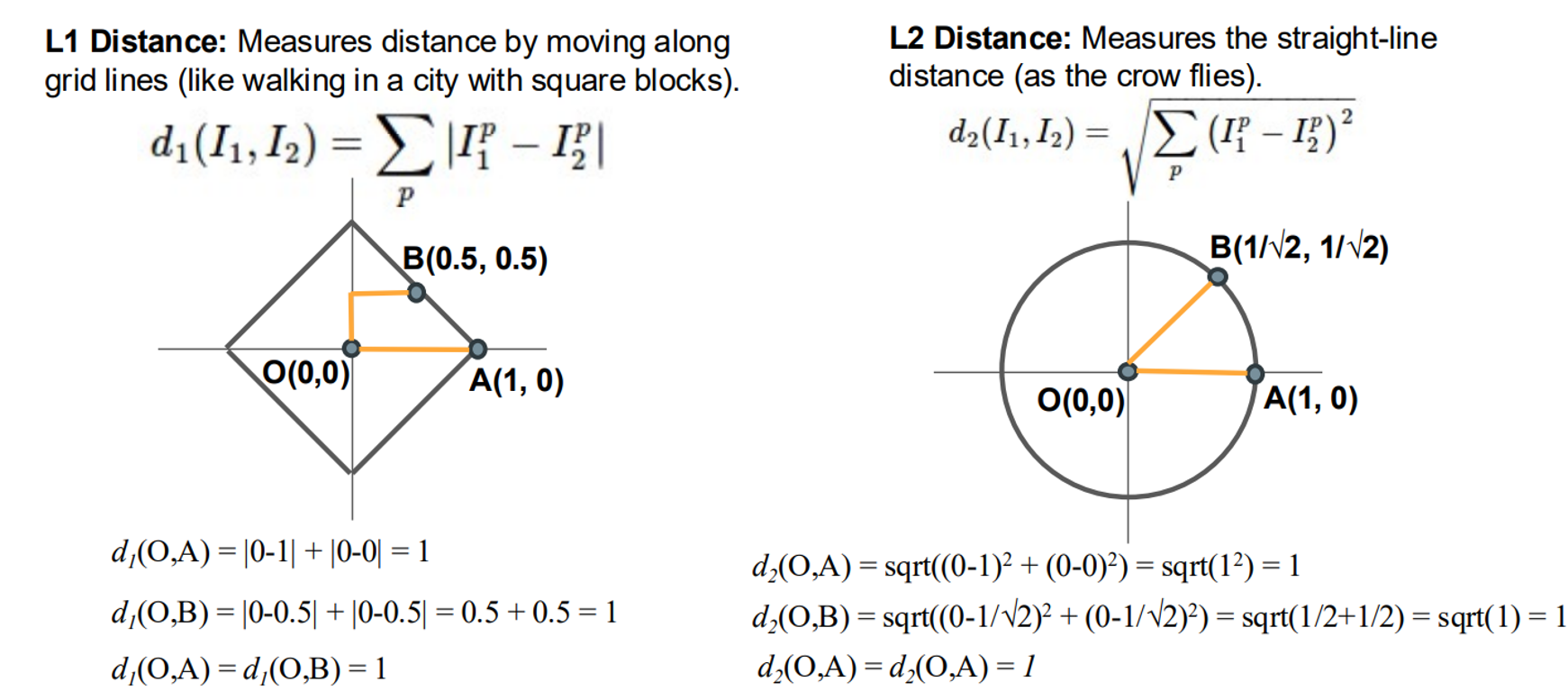
• L1 Distance (Manhattan Distance): This calculates the sum of the absolute differences between the corresponding pixel values of two images. $d_1(I_1, I_2) = \sum_p |I_1^p - I_2^p|$ Imagine walking in a city: you move along grid lines (horizontally or vertically).

• L2 Distance (Euclidean Distance): This calculates the square root of the sum of the squared differences between the corresponding pixel values. $d_2(I_1, I_2) = \sqrt{\sum_p (I_1^p - I_2^p)^2}$ This is like the straight-line distance “as the crow flies”.

Hyperparameters and Their Tuning

In KNN, K (the number of neighbors) and the choice of distance metric (L1 or L2) are hyperparameters. These are choices about the algorithm itself, and their optimal values are highly dependent on the specific problem and dataset.

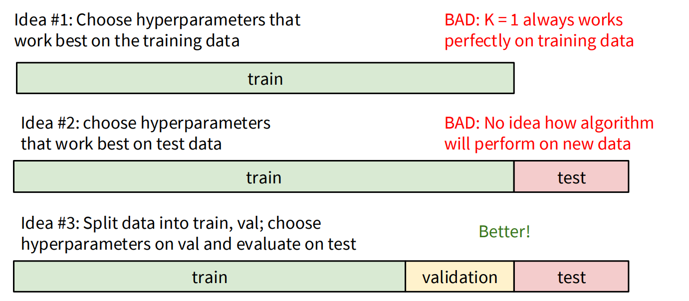
To find the best hyperparameters, we use a strategy involving data splitting:

1. Avoid Training Set Tuning: Choosing hyperparameters that work best on the training data is a bad idea because K=1 will always yield perfect accuracy on the training set (it just finds itself!). This leads to overfitting.
2. Avoid Test Set Tuning: Using the test set to tune hyperparameters is also problematic because it gives an unrealistic estimate of how the algorithm will perform on truly new, unseen data. You should only run on the test set once at the very end.
3. Validation Set: The recommended approach is to split your data into three sets:
   • Training set: Used to train the model.
   • Validation set: Used to tune hyperparameters. You experiment with different K values and distance metrics on this set.
   • Test set: Used for the final evaluation of the model’s performance on completely unseen data.

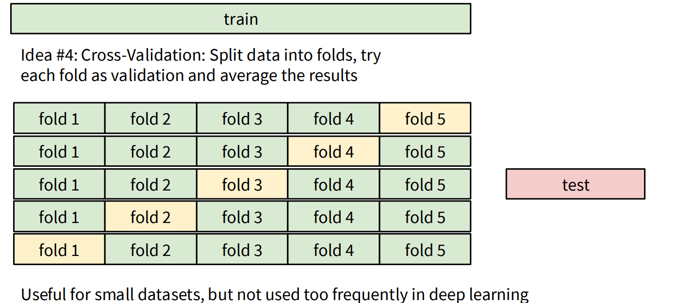
4. Cross-Validation: For smaller datasets, k-fold cross-validation is a robust method where the training data is split into ‘k’ folds. Each fold takes a turn as the validation set, and the results are averaged. This is less common in deep learning due to the large dataset sizes.

Limitations of KNN

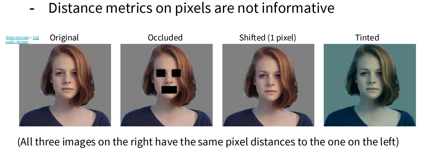
While simple, KNN has limitations, especially when using pixel distances directly:

• Pixel distances are not always informative. Small shifts, occlusions, or changes in lighting can drastically alter pixel values, making images that are perceptually similar appear very different to the algorithm based on simple pixel-wise distance.

Conceptual KNN Implementation (Python/NumPy)

While PyTorch is primarily for neural networks, we can conceptualize the KNN logic. Typically, KNN would be implemented using libraries like scikit-learn. Here’s a conceptual Python implementation using NumPy for demonstration of the L1 distance:

import numpy as np

class KNearestNeighbor:
    def __init__(self):
        pass

    def train(self, X, y):
        """
        Train the classifier. For K-nearest neighbors, this
        simply stores the training data.
        :param X: A numpy array of shape (N, D) containing N
                  training examples each of dimension D.
        :param y: A numpy array of shape (N,) containing the training labels.
        """
        self.X_train = X
        self.y_train = y

    def predict(self, X):
        """
        Predict labels for test data using this classifier.
        :param X: A numpy array of shape (N_test, D) containing N_test
                  test examples each of dimension D.
        :return: A numpy array of shape (N_test,) containing the predicted labels for the
                 test data.
        """
        num_test = X.shape[0]
        num_train = self.X_train.shape[0]
        Y_pred = np.zeros(num_test, dtype=self.y_train.dtype)

        # Using L1 distance for simplicity (Manhattan Distance)
        # It's more efficient to do this with broadcasting, but for clarity, a loop.
        for i in range(num_test):
            # Compute L1 distance between the i-th test point and all training points
            distances = np.sum(np.abs(self.X_train - X[i, :]), axis=1)
            min_idx = np.argmin(distances)
            Y_pred[i] = self.y_train[min_idx]

        return Y_pred

# Example Usage (conceptual - you'd replace with actual image data)
# X_train_sample = np.random.rand(100, 32*32*3) # 100 images, 32x32 RGB
# y_train_sample = np.random.randint(0, 10, 100) # 10 classes
# X_test_sample = np.random.rand(10, 32*32*3) # 10 test images

# knn = KNearestNeighbor()
# knn.train(X_train_sample, y_train_sample)
# predictions = knn.predict(X_test_sample)
# print(predictions)

Linear Classifier

The Linear Classifier takes a different, parametric approach. Instead of memorizing data, it learns a set of parameters (weights) that allow it to compute scores for each class based on the input image.

How Linear Classifier Works

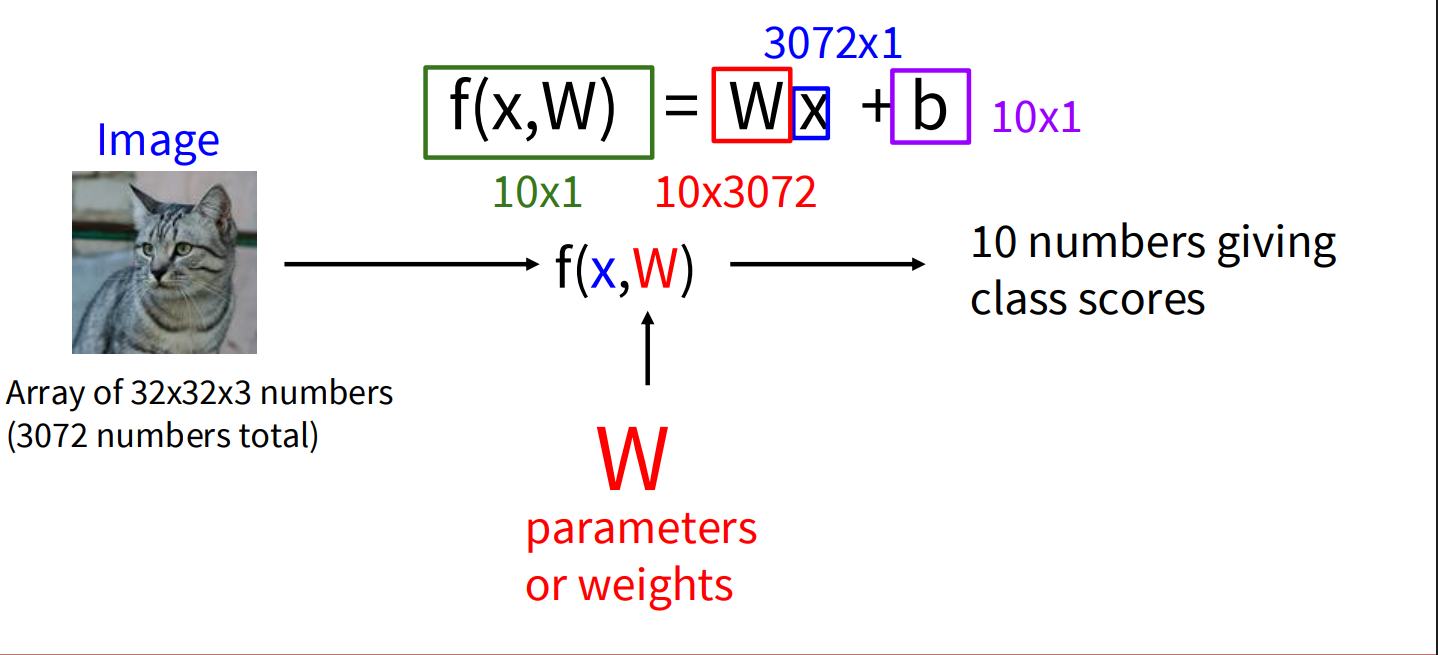
A linear classifier computes class scores for an image using a linear function. For an input image represented as a vector x and a set of learnable parameters (weights) W and biases b, the scores are calculated as: $f(x, W) = Wx + b$

• x: The input image, flattened into a single column vector of pixel values. For a 32x32x3 (width x height x channels) image, this would be a 3072x1 vector.
• W: The weight matrix. If you have C classes, and your input image has D dimensions (e.g., 3072), then W will be a C x D matrix (e.g., 10x3072 for CIFAR-10). Each row of W corresponds to a specific class.
• b: The bias vector. This is a C x 1 vector (e.g., 10x1).

The result, f(x, W), is a C x 1 vector where each element represents the score for a particular class. The class with the highest score is the predicted label.

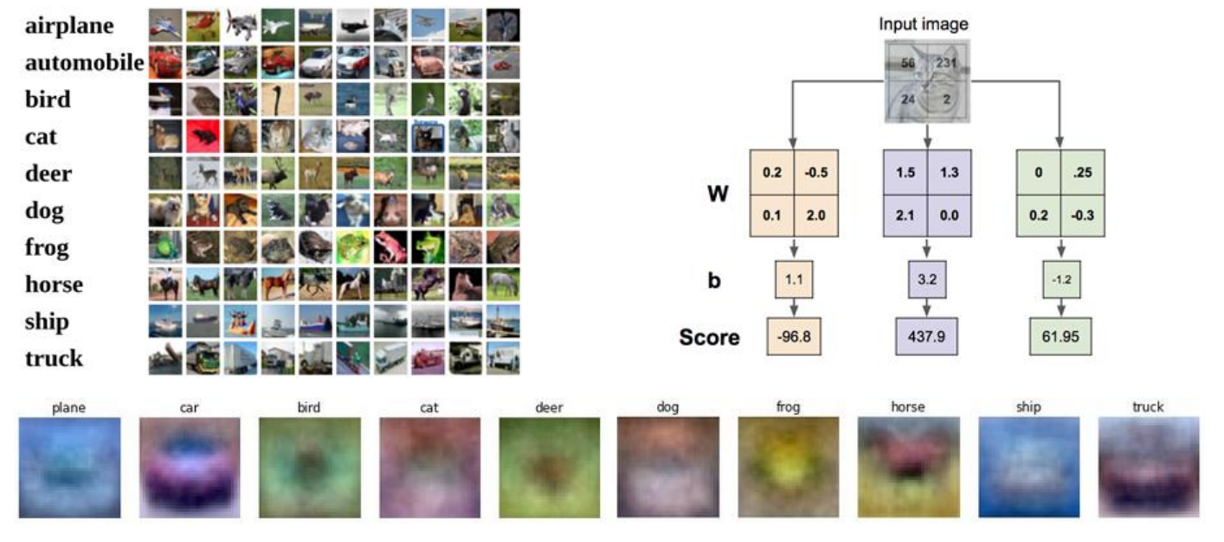
Interpreting the Weights (W)

Each row of the weight matrix W can be thought of as a “template” or “prototype” for a specific class. When you compute Wx, you are essentially performing a dot product (or similarity measure) between the input image and each of these class templates. The bias b allows the model to shift these scores independently for each class.

Simple Linear Classifier in PyTorch

PyTorch is well-suited for implementing linear classifiers (and much more complex neural networks).

import torch
import torch.nn as nn

# Assume a flattened image input (e.g., 32x32x3 = 3072 features)
input_features = 3072
num_classes = 10 # For example, CIFAR-10 has 10 classes

# Define a simple Linear Classifier model
class LinearClassifier(nn.Module):
    def __init__(self, input_dim, num_classes):
        super(LinearClassifier, self).__init__()
        # nn.Linear creates a layer that applies a linear transformation: y = xA^T + b
        self.linear = nn.Linear(input_dim, num_classes)

    def forward(self, x):
        # Flatten the input image if it's not already flattened
        # For a batch of images, reshape from (batch_size, channels, height, width)
        # to (batch_size, channels * height * width)
        x = x.view(x.size(0), -1) # -1 infers the dimension
        scores = self.linear(x)
        return scores

# --- Example Usage (Conceptual) ---
# Create a dummy batch of images (e.g., 4 images, each 3x32x32)
# In a real scenario, these would come from a DataLoader
# dummy_images = torch.randn(4, 3, 32, 32) # Batch size 4, 3 channels, 32x32 pixels

# Instantiate the model
# model = LinearClassifier(input_features, num_classes)

# Get raw scores from the model
# raw_scores = model(dummy_images)
# print("Raw scores for each image and class:\n", raw_scores)

# To get the predicted class, we typically take the argmax of the scores
# This gives the index of the highest score for each image in the batch
# predicted_classes = torch.argmax(raw_scores, dim=1)
# print("\nPredicted classes for each image:\n", predicted_classes)

Training a Linear Classifier on CIFAR-10 with PyTorch and Visualizing Weights

Now, let’s put the linear classifier into action by training one on the CIFAR-10 dataset and then visualizing the learned weight parameters.

Setting up the Environment and Data

First, we need to import necessary libraries and load the CIFAR-10 dataset using torchvision. We’ll also define data transformations to normalize the pixel values.

import torch
import torch.nn as nn
import torch.optim as optim
import torchvision
import torchvision.transforms as transforms
from torch.utils.data import DataLoader
import numpy as np
import matplotlib.pyplot as plt

# Check if CUDA is available, otherwise use CPU
device = torch.device("cuda" if torch.cuda.is_available() else "cpu")
print(f"Using device: {device}")

# Define data transformations for training and testing
transform_train = transforms.Compose([
    transforms.ToTensor(),
    transforms.Normalize((0.5, 0.5, 0.5), (0.5, 0.5, 0.5)) # Normalize to [-1, 1]
])

transform_test = transforms.Compose([
    transforms.ToTensor(),
    transforms.Normalize((0.5, 0.5, 0.5), (0.5, 0.5, 0.5))
])

# Load the CIFAR-10 training dataset
trainset = torchvision.datasets.CIFAR10(root='./data', train=True,
                                        download=True, transform=transform_train)
trainloader = DataLoader(trainset, batch_size=64,
                          shuffle=True, num_workers=2)

# Load the CIFAR-10 testing dataset
testset = torchvision.datasets.CIFAR10(root='./data', train=False,
                                       download=True, transform=transform_test)
testloader = DataLoader(testset, batch_size=64,
                         shuffle=False, num_workers=2)

# Define the 10 classes in CIFAR-10
classes = ('plane', 'car', 'bird', 'cat',
           'deer', 'dog', 'frog', 'horse', 'ship', 'truck')

Defining the Linear Classifier Model (Instantiated)

We instantiate the LinearClassifier class for the CIFAR-10 dataset.

# Instantiate the model
input_features = 32 * 32 * 3 # CIFAR-10 images are 32x32 with 3 color channels
num_classes = 10
model = LinearClassifier(input_features, num_classes).to(device)

Defining Loss Function and Optimizer

We’ll use the Cross-Entropy Loss, which is standard for multi-class classification, and the Stochastic Gradient Descent (SGD) optimizer.

# Define the loss function
criterion = nn.CrossEntropyLoss()

# Define the optimizer
optimizer = optim.SGD(model.parameters(), lr=0.001, momentum=0.9)

The Training Loop

Now, we implement the main training loop. We’ll iterate through the training data for a specified number of epochs. In each epoch, we’ll perform a forward pass, calculate the loss, perform a backward pass to compute gradients, and then update the model’s weights using the optimizer.

# Training the model
num_epochs = 10
print("Starting training...")
for epoch in range(num_epochs):
    running_loss = 0.0
    for i, data in enumerate(trainloader, 0):
        inputs, labels = data
        inputs, labels = inputs.to(device), labels.to(device)

        # Zero the parameter gradients
        optimizer.zero_grad()

        # Forward pass
        outputs = model(inputs)
        loss = criterion(outputs, labels)

        # Backward pass and optimize
        loss.backward()
        optimizer.step()

        # Print statistics
        running_loss += loss.item()
        if i % 2000 == 1999:    # Print every 2000 mini-batches
            print(f'[{epoch + 1}, {i + 1:5d}] loss: {running_loss / 2000:.3f}')
            running_loss = 0.0

print('Finished Training')

Evaluating the Model

It’s good practice to evaluate the model’s performance on the test set after training.

# Evaluate the model on the test set
correct = 0
total = 0
with torch.no_grad():
    for data in testloader:
        images, labels = data
        images, labels = images.to(device), labels.to(device)
        outputs = model(images)
        _, predicted = torch.max(outputs.data, 1)
        total += labels.size(0)
        correct += (predicted == labels).sum().item()

print(f'\nAccuracy of the network on the 10000 test images: {100 * correct / total:.2f} %')

# Class-wise accuracy
class_correct = list(0. for i in range(10))
class_total = list(0. for i in range(10))
with torch.no_grad():
    for data in testloader:
        images, labels = data
        images, labels = images.to(device), labels.to(device)
        outputs = model(images)
        _, predicted = torch.max(outputs, 1)
        c = (predicted == labels).squeeze()
        for i in range(len(labels)):
            label = labels.cpu().numpy()[i]
            class_correct[label] += c.cpu().numpy()[i]
            class_total[label] += 1

print('\nAccuracy per class:')
for i in range(10):
    if class_total[i] > 0: # Avoid division by zero
        print(f'Accuracy of {classes[i]}: {100 * class_correct[i] / class_total[i]:.2f} %')
    else:
        print(f'No test samples for {classes[i]}')

Visualizing the Learned Weights

Now comes the interesting part: visualizing the weights learned by the linear layer. Each row in the weight matrix W (of size num_classes x input_features) corresponds to a class. We can reshape each row back into an image of the original size (3x32x32) and visualize it.

# Get the learned weights from the linear layer
linear_layer = model.linear
weights = linear_layer.weight.detach().cpu().numpy()

# Visualize the weights for each class
fig, axes = plt.subplots(2, 5, figsize=(10, 4))
fig.suptitle('Learned Weights as Class Templates')
for i, ax in enumerate(axes.ravel()):
    # Get the weight vector for the i-th class
    weight_vector = weights[i, :]
    # Reshape it to the original image dimensions (3x32x32)
    weight_image = weight_vector.reshape(3, 32, 32)
    # Transpose to (32, 32, 3) for proper image display and normalize to [0, 1]
    # We normalize each image independently to ensure proper visualization
    weight_image = np.transpose(weight_image, (1, 2, 0))
    # Normalize to [0, 1] for visualization
    weight_image = (weight_image - weight_image.min()) / (weight_image.max() - weight_image.min() + 1e-8) # Add small epsilon to avoid div by zero

    # Display the weight as an image
    ax.imshow(weight_image)
    ax.set_title(classes[i])
    ax.axis('off')

plt.tight_layout(rect=[0, 0.03, 1, 0.95]) # Adjust layout to prevent title overlap
plt.show()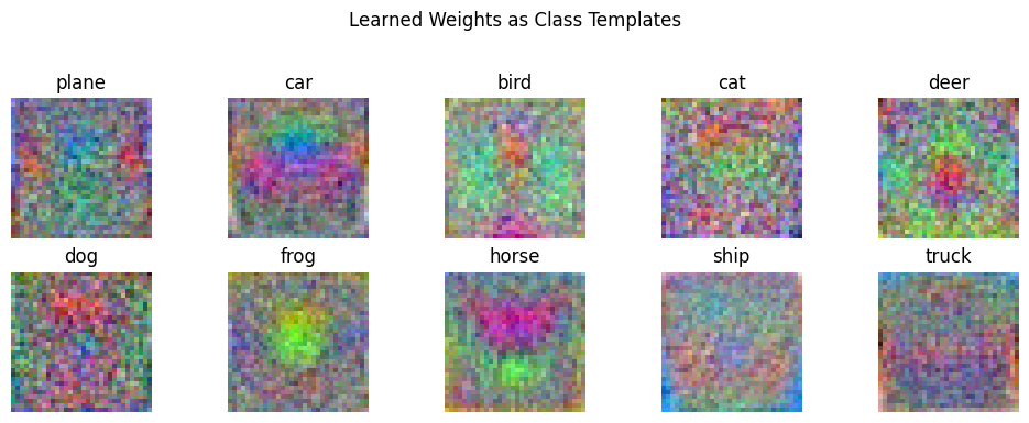

Explanation of Weight Visualization:

The visualized weights can sometimes provide insights into what the linear classifier has learned to associate with each class. Ideally, for each class, the corresponding weight visualization might show a blurry or noisy template of the objects belonging to that class.

• Each of the 10 subplots represents the learned weights for one of the CIFAR-10 classes.
• The pixel intensities in these weight visualizations indicate the “importance” of those pixels for that particular class.
• Positive weight values for a pixel suggest that a high intensity in that pixel contributes positively to the score of that class.
• Negative weight values suggest that a high intensity in that pixel detracts from the score of that class.

Important Note:

Keep in mind that linear classifiers are quite limited in their ability to learn complex visual features directly from raw pixels. The visualizations might appear noisy or not perfectly representative of the class objects. More sophisticated models like Convolutional Neural Networks (CNNs) are much better at learning meaningful hierarchical features from images, and their weight visualizations (especially in the earlier layers) tend to be more interpretable in terms of edges, textures, and basic shapes.

Conclusion

This example provides a fundamental understanding of the training process for a simple linear classifier in PyTorch and a basic way to inspect the learned parameters. As you move towards more complex models, the training loop structure will remain similar, but the model architecture and the interpretation of learned features will become more intricate. The journey from simple pixel-wise comparisons to learning complex visual hierarchies is what makes deep learning for image classification so powerful.

---