Deep Learning - From Perceptrons to Practical Training

(Adopted from MIT 6.S191 - Introduction to Deep Learning)

Deep Learning: From Perceptrons to Practical Training

This blog post provides a comprehensive introduction to neural networks and deep learning, covering foundational concepts such as perceptrons, activation functions, loss minimization, and practical training techniques. Code examples in PyTorch are included to illustrate key concepts.

1. Introduction to Deep Learning

Deep learning, a subset of machine learning, involves teaching computers to learn directly from raw data by extracting patterns using neural networks. This approach mimics human behavior to enable computers to learn without explicit programming.

Over the years, the progress in deep learning has been remarkable. For instance, creating a two-minute video in 2020 required significant resources (2 hours of professional audio, 50 hours of HD video, a static script, and over $15K USD in compute), with expectations for even faster and more efficient generation in the future.

Deep learning has gained dominance recently due to three main factors:

• Big Data: The availability of larger datasets and easier data collection and storage.
• Hardware: The advent of Graphics Processing Units (GPUs) that allow for massively parallelizable computations.
• Software: Improved techniques, new models, and robust toolboxes (like TensorFlow and PyTorch).

2. Prerequisites for this Course

To understand deep learning effectively, it’s helpful to have a grasp of the following prerequisites:

• Basic Python (Numpy, Pandas)
• Linear Algebra (Vector, Matrix, Tensor)
• Statistics & Probability
• Optimization Theories
• Classical Machine Learning (Supervised: Linear and Logistic Regression; Unsupervised: Clustering)

3. Recap: Linear vs. Logistic Regression

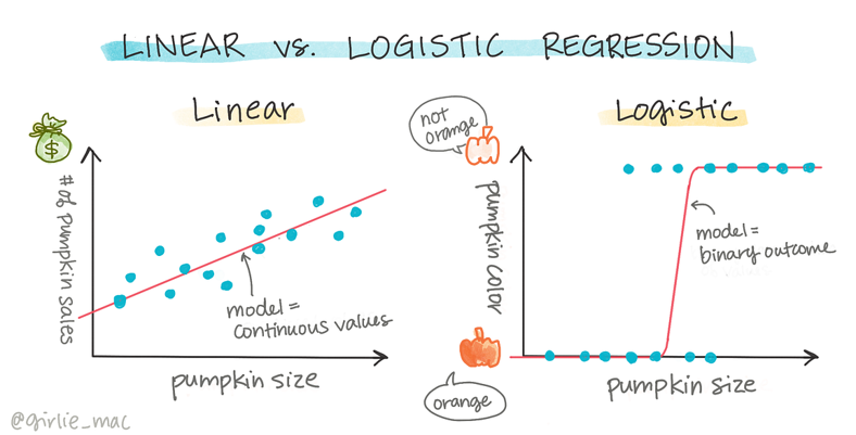
Linear Regression

Linear regression is used for predicting continuous values. It aims to fit a line that minimizes the prediction error.

• Type: Regression (predicts continuous values)
• Model Equation: $\hat{y} = \beta_0 + \beta_1x_1 + \cdots + \beta_px_p$
• Goal: Fit a line that minimizes the prediction error
• Loss Function: Mean Squared Error (MSE): $L(\mathbf{\beta}) = \frac{1}{n} \sum_{i=1}^{n} (y_i - \hat{y}_i)^2$
• Optimization: Closed-form solution via Normal Equation or Gradient Descent

Logistic Regression

Logistic regression is used for classification tasks, predicting the probability of class membership. It fits an S-shaped curve to estimate class probability.

• Type: Classification (predicts probability for class membership)
• Model Equation: $z = \beta_0 + \beta_1x_1 + \cdots + \beta_px_p$; $p_1 = \hat{y} = \frac{1}{1 + e^{-z}}$
• Goal: Fit an S-shaped curve that estimates class probability
• Loss Function: Binary Cross-Entropy (Log Loss)
• Optimization: Typically solved using Gradient Descent

4. Perceptron: The Building Block

The perceptron is the fundamental building block of neural networks. It takes multiple inputs, applies weights to them, sums them up, and then passes the result through a non-linear activation function to produce an output.

The process of feeding input into the network and obtaining an output is known as a ‘forward pass’ or ‘forward propagation’.

• Equation: $\hat{y} = g(w_0 + \mathbf{X}^T\mathbf{W})$
  • $w_0$: Bias
  • $\mathbf{X}$: Inputs vector
  • $\mathbf{W}$: Weights vector
  • $g$: Non-linear activation function

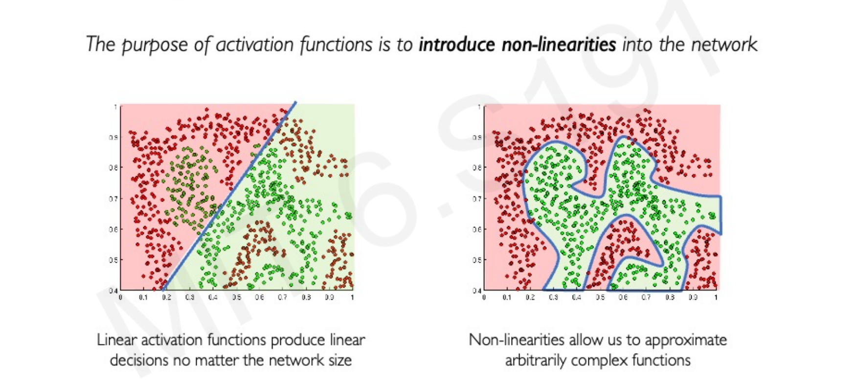
Activation Functions

Activation functions introduce non-linearities into the network, enabling it to approximate arbitrarily complex functions. Without non-linear activation functions, a neural network, regardless of its size, would only be capable of linear decisions.

Common activation functions include:

• Sigmoid Function: $g(z) = \frac{1}{1 + e^{-z}}$
  • Derivative: $g'(z) = g(z)(1 - g(z))$
  • PyTorch: torch.sigmoid(z)
• Hyperbolic Tangent (Tanh): $g(z) = \frac{e^z - e^{-z}}{e^z + e^{-z}}$
  • Derivative: $g'(z) = 1 - g(z)^2$
  • PyTorch: torch.tanh(z)
• Rectified Linear Unit (ReLU): $g(z) = \max(0, z)$
  • Derivative: $g'(z) = 1$ if $z > 0$, and $0$ otherwise
  • PyTorch: torch.nn.ReLU()

5. From Perceptron to Neural Network

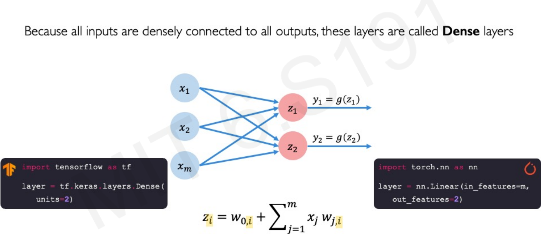
A Multivariate Perceptron (or a dense layer) consists of multiple perceptrons where all inputs are densely connected to all outputs.

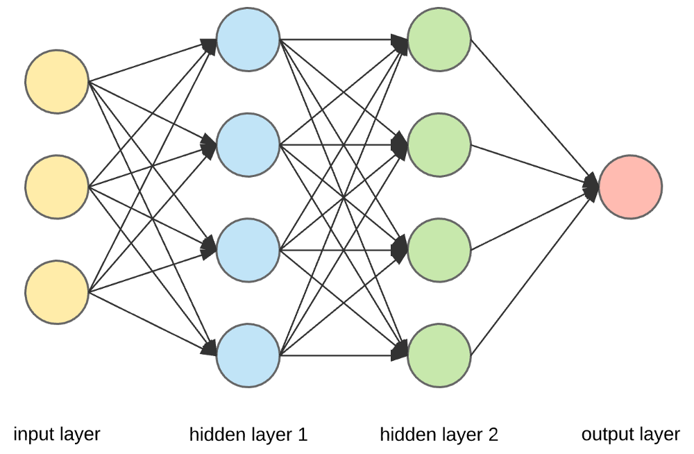
A Neural Network is formed by stacking multiple perceptrons, creating hidden layers between the input and output layers. When a neural network has many hidden layers, it is referred to as a Deep Neural Network.

Here’s how to define dense layers and sequential models in PyTorch:

import torch
import torch.nn as nn

# Example for a single dense layer (Multivariate Perceptron)
# input_features is 'm', output_features is 'n' (number of perceptrons in the layer)
m = 4  # Example input features
n = 3  # Example output features for the first hidden layer

# A single dense layer (Linear layer in PyTorch)
layer = nn.Linear(m, n)
print(layer)
# Example of forward pass for a single layer
input_tensor = torch.randn(1, m) # Batch size of 1, m input features
output_tensor = layer(input_tensor)
print(f"Output of single layer: {output_tensor.shape}")

# From Perceptron to Neural Network (a simple two-layer network)
# Here, we'll define a model with one hidden layer and an output layer
# Assuming 'm' input features, 'n_hidden' neurons in the hidden layer, and 'n_output' output neurons

n_hidden = 5  # Number of neurons in the hidden layer
n_output = 2  # Number of output neurons

model_nn = nn.Sequential(
    nn.Linear(m, n_hidden),  # Input layer to hidden layer
    nn.ReLU(),               # Activation function
    nn.Linear(n_hidden, n_output) # Hidden layer to output layer
)
print(f"\nSimple Neural Network (2 layers):\n{model_nn}")

# Example of a forward pass through the neural network
output_nn = model_nn(input_tensor)
print(f"Output of Neural Network: {output_nn.shape}")

# From Neural Network to Deep Neural Network (multiple hidden layers)
# Let's add more hidden layers to make it a deep neural network
nk = 10 # Number of neurons in the second hidden layer

model_dnn = nn.Sequential(
    nn.Linear(m, n_hidden),  # First hidden layer
    nn.ReLU(),
    nn.Linear(n_hidden, nk), # Second hidden layer
    nn.ReLU(),
    nn.Linear(nk, n_output)  # Output layer
)
print(f"\nDeep Neural Network (3 hidden layers):\n{model_dnn}")

# Example of a forward pass through the deep neural network
output_dnn = model_dnn(input_tensor)
print(f"Output of Deep Neural Network: {output_dnn.shape}")

6. Loss Function

The loss function quantifies the cost incurred from incorrect predictions by the network. The goal of training a neural network is to find the network weights ($W$) that achieve the lowest loss.

The empirical loss measures the total loss over the entire dataset: $J(\mathbf{W}) = \frac{1}{n} \sum_{i=1}^{n} \mathcal{L}(f(\mathbf{x}^{(i)}; \mathbf{W}), y^{(i)})$ where:

• $f(\mathbf{x}^{(i)}; \mathbf{W})$ is the predicted output
• $y^{(i)}$ is the actual output

Binary Cross-Entropy Loss

Binary Cross-Entropy loss is typically used with models that output a probability between 0 and 1, common in binary classification tasks.

• Formula: $J(\mathbf{W}) = -\frac{1}{n} \sum_{i=1}^{n} [y^{(i)}\log(f(\mathbf{x}^{(i)}; \mathbf{W})) + (1 - y^{(i)})\log(1 - f(\mathbf{x}^{(i)}; \mathbf{W}))]$
• PyTorch Implementation: torch.nn.functional.binary_cross_entropy(predicted, target)

Mean Squared Error (MSE)

Mean Squared Error loss is used for regression models that output continuous real numbers.

• Formula: $J(\mathbf{W}) = \frac{1}{n} \sum_{i=1}^{n} (y^{(i)} - f(\mathbf{x}^{(i)}; \mathbf{W}))^2$
• PyTorch Implementation: torch.nn.functional.mse_loss(predicted, target)

import torch
import torch.nn as nn
import torch.nn.functional as F

# Example data for loss calculation
predicted_proba = torch.tensor([0.1, 0.8, 0.6]) # Predicted probabilities
actual_binary = torch.tensor([1.0, 0.0, 1.0])   # Actual binary labels

# Binary Cross-Entropy Loss
bce_loss = F.binary_cross_entropy(predicted_proba, actual_binary)
print(f"\nBinary Cross-Entropy Loss: {bce_loss.item()}")

# Example data for MSE calculation
predicted_grades = torch.tensor([30.0, 80.0, 85.0]) # Predicted continuous values
actual_grades = torch.tensor([90.0, 20.0, 95.0])    # Actual continuous values

# Mean Squared Error Loss
mse_loss = F.mse_loss(predicted_grades, actual_grades)
print(f"Mean Squared Error Loss: {mse_loss.item()}")

7. Loss Minimization: Gradient Descent

The process of finding the optimal weights ($W^*$) that minimize the loss function $J(W)$ is typically done using Gradient Descent.

The algorithm for Gradient Descent involves:

1. Initialize weights randomly, often from a normal distribution $\mathcal{N}(0, \sigma^2)$.
2. Loop until convergence:
   • Compute the gradient of the loss function with respect to the weights, $\frac{\partial J(\mathbf{W})}{\partial \mathbf{W}}$.
   • Update the weights: $\mathbf{W} \leftarrow \mathbf{W} - \eta \frac{\partial J(\mathbf{W})}{\partial \mathbf{W}}$, where $\eta$ is the learning rate.
3. Return the optimized weights.

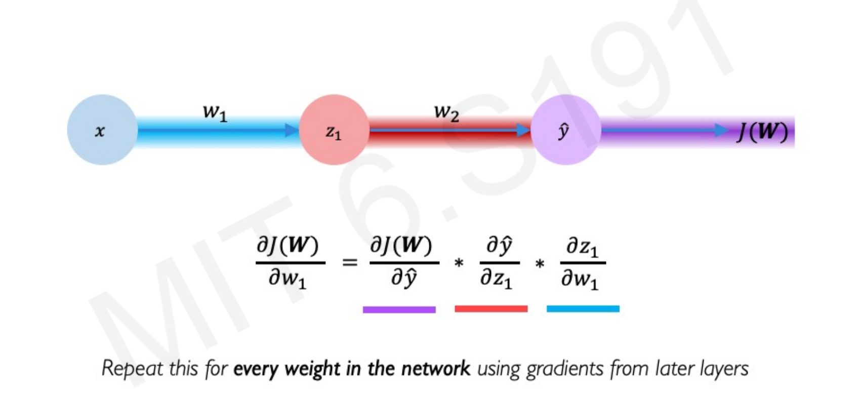
Computing Gradients (Backpropagation): Gradients are computed by applying the chain rule, propagating the error backward through the network to determine how much each weight contributed to the overall loss. This process is known as backpropagation.

Learning Rate ($\eta$): The learning rate determines the size of the steps taken during weight updates. Historically, learning rates were fixed, but modern approaches use adaptive learning rates. Adaptive learning rates can be adjusted (made larger or smaller) based on factors like the magnitude of the gradient, the speed of learning, or the size of particular weights.

Gradient Descent Variants

Several variants of gradient descent exist, each with its own optimization strategy:

• SGD (Stochastic Gradient Descent): torch.optim.SGD
• Adam: torch.optim.Adam
• Adadelta: torch.optim.Adadelta
• Adagrad: torch.optim.Adagrad
• RMSProp: torch.optim.RMSprop

import torch
import torch.nn as nn
import torch.optim as optim

# Define a simple neural network for demonstration
class SimpleNN(nn.Module):
    def __init__(self):
        super(SimpleNN, self).__init__()
        self.linear = nn.Linear(10, 1) # 10 input features, 1 output

    def forward(self, x):
        return self.linear(x)

model = SimpleNN()
criterion = nn.MSELoss() # Mean Squared Error as loss function
optimizer = optim.SGD(model.parameters(), lr=0.01) # Stochastic Gradient Descent optimizer

# Dummy data
inputs = torch.randn(5, 10) # 5 samples, 10 features
targets = torch.randn(5, 1) # 5 samples, 1 output

# Training loop (simplified)
num_epochs = 100
for epoch in range(num_epochs):
    optimizer.zero_grad() # Clear gradients
    outputs = model(inputs)
    loss = criterion(outputs, targets)
    loss.backward() # Compute gradients
    optimizer.step() # Update weights

    if (epoch+1) % 10 == 0:
        print(f'Epoch [{epoch+1}/{num_epochs}], Loss: {loss.item():.4f}')

# Example of different optimizers
adam_optimizer = optim.Adam(model.parameters(), lr=0.001)
adagrad_optimizer = optim.Adagrad(model.parameters(), lr=0.01)

8. Mini-Batch Training

Instead of computing gradients over the entire dataset (which can be slow for large datasets), mini-batch training computes gradients on small subsets (batches) of data. This leads to faster training and allows for parallel computation, especially on GPUs.

The algorithm for mini-batch training is similar to gradient descent but with an added step to pick a batch of data points:

1. Initialize weights randomly.
2. Loop until convergence:
   • Pick a batch of $B$ data points.
   • Compute gradient for the batch.
   • Update weights.
3. Return weights.

9. Overfitting and Regularization

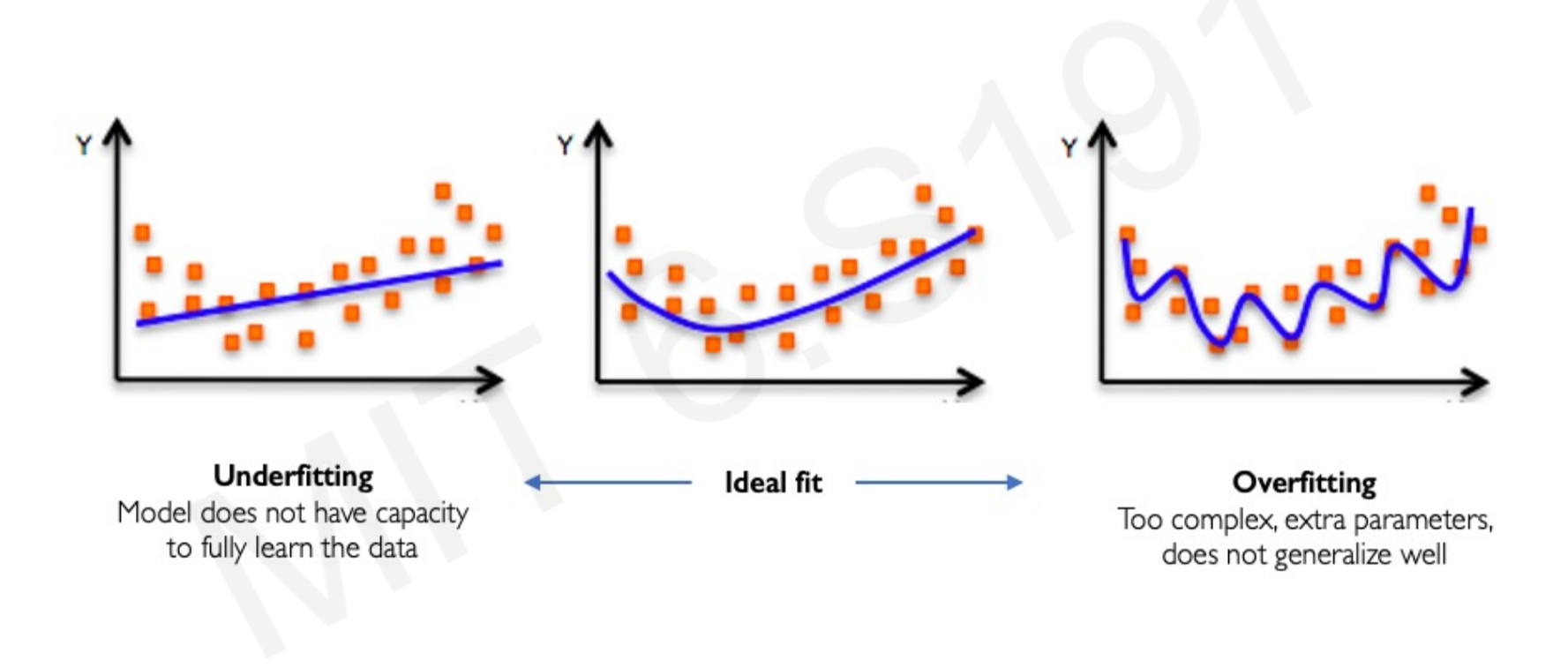
Overfitting occurs when a model learns the training data too well, capturing noise and specific patterns that do not generalize to new, unseen data. This results in poor performance on test data. Conversely, underfitting happens when the model is too simple to capture the underlying patterns in the data. An ideal fit strikes a balance between underfitting and overfitting.

To combat overfitting, regularization techniques are employed.

Regularization I: Dropout

Dropout is a regularization technique where, during training, a random proportion (typically 50%) of activations in a layer are set to zero. This forces the network to not rely on any single node, making it more robust and preventing co-adaptation of neurons.

• PyTorch Implementation: torch.nn.Dropout(p=0.5)

import torch
import torch.nn as nn

# Define a neural network with Dropout layers
class DropoutNN(nn.Module):
    def __init__(self):
        super(DropoutNN, self).__init__()
        self.linear1 = nn.Linear(10, 20)
        self.relu = nn.ReLU()
        self.dropout = nn.Dropout(p=0.5) # Dropout with 50% probability
        self.linear2 = nn.Linear(20, 1)

    def forward(self, x):
        x = self.linear1(x)
        x = self.relu(x)
        x = self.dropout(x) # Apply dropout
        x = self.linear2(x)
        return x

model_dropout = DropoutNN()
print(f"\nModel with Dropout:\n{model_dropout}")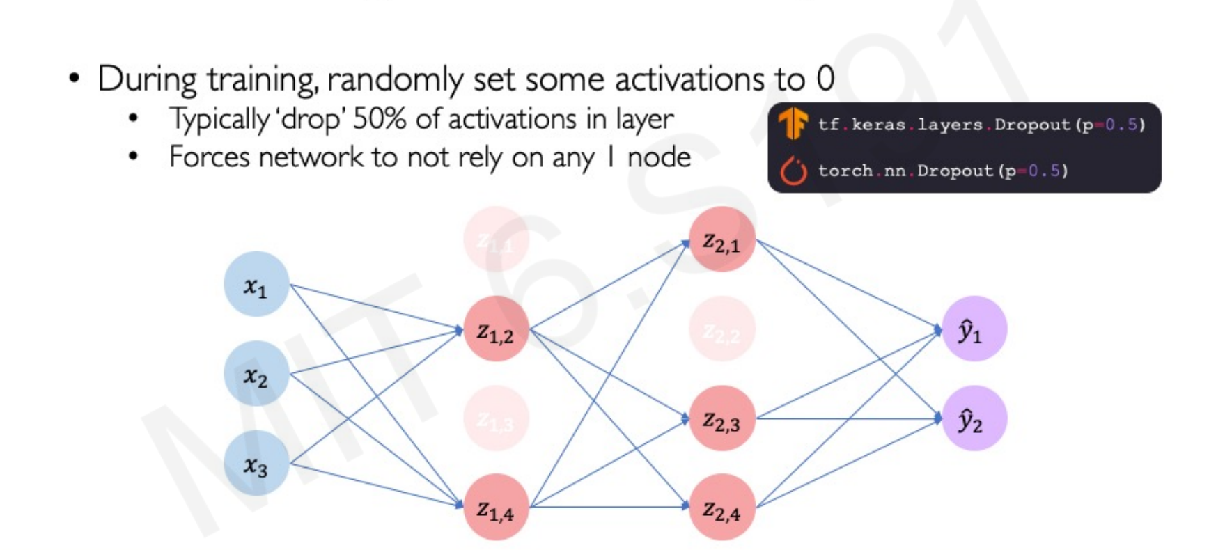

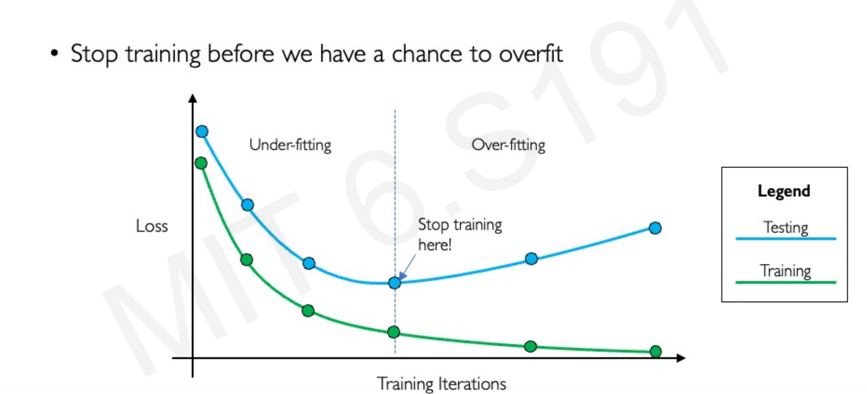
Regularization II: Early Stopping

Early stopping is a regularization technique where training is stopped before the model has a chance to overfit. This is typically done by monitoring the model’s performance on a validation set and stopping training when the validation loss starts to increase, even if the training loss is still decreasing.

10. Summary

In summary, this tutorial covered:

• The Perceptron: The structural building block of neural networks, incorporating non-linear activation functions.
• Neural Networks: Formed by stacking perceptrons, with optimization achieved through backpropagation.
• Training in Practice: Key concepts include adaptive learning rates, mini-batch training, and regularization techniques like dropout and early stopping.