A Gentle Introduction to Continuous Optimization

Published on Thursday, 21-08-2025

#Tutorials

(Adopted from CS221)

image info

🌐 A Gentle Introduction to Continuous Optimization

Optimization is at the heart of modern data science, machine learning, and applied mathematics. Continuous optimization deals with problems where the variables can take on any real value (as opposed to discrete optimization, where variables are integers or categorical).

In this tutorial, we’ll explore the fundamentals of continuous optimization, step-by-step, with math, Python code, and visualizations.

🔹 1. What is Continuous Optimization?

Formally, an optimization problem looks like:

\min_{x \in \mathbb{R}^n} f(x)

Where:

$f(x)$ is the objective function (real-valued, differentiable in most cases).
$x \in \mathbb{R}^n$ is the vector of decision variables.

If there are constraints, the problem becomes:

\begin{aligned} \min_{x \in \mathbb{R}^n} & \quad f(x) \\ \text{subject to:} & \quad g_i(x) \leq 0, \; i=1,\dots,m \\ & \quad h_j(x) = 0, \; j=1,\dots,p \end{aligned}

$g_i(x)$ : inequality constraints
$h_j(x)$ : equality constraints

🔹 2. Gradient Descent: The Core Idea

The simplest and most widely used method for continuous optimization is gradient descent.

The update rule is:

x^{(k+1)} = x^{(k)} - \eta \nabla f(x^{(k)})

Where:

$\eta > 0$ is the learning rate.
$\nabla f(x)$ is the gradient (vector of partial derivatives).

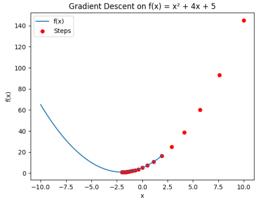
🔹 Example: Minimizing a Quadratic Function

Let’s minimize:

f(x) = x^2 + 4x + 5

The derivative is:

f'(x) = 2x + 4

🔹 3. Python Implementation

import numpy as np
import matplotlib.pyplot as plt

# Objective function
def f(x):
    return x**2 + 4*x + 5

# Gradient
def grad_f(x):
    return 2*x + 4

# Gradient descent
x = 10.0   # initial point
eta = 0.1  # learning rate
history = [x]

for _ in range(30):
    x = x - eta * grad_f(x)
    history.append(x)

# Visualization
x_vals = np.linspace(-10, 2, 200)
y_vals = f(x_vals)

plt.plot(x_vals, y_vals, label="f(x)")
plt.scatter(history, [f(h) for h in history], color='red', s=30, label="Steps")
plt.title("Gradient Descent on f(x) = x² + 4x + 5")
plt.xlabel("x")
plt.ylabel("f(x)")
plt.legend()
plt.show()

✅ This will show how gradient descent iteratively approaches the minimum.

🔹 4. Multivariate Case

For $f(x, y)$ , the gradient is:

\nabla f(x,y) = \begin{bmatrix} \frac{\partial f}{\partial x} \\ \frac{\partial f}{\partial y} \end{bmatrix}

Example:

f(x, y) = x^2 + y^2

The gradient is:

\nabla f(x,y) = \begin{bmatrix} 2x \\ 2y \end{bmatrix}

Python Visualization

# Multivariate Gradient Descent
def f_xy(x, y):
    return x**2 + y**2

def grad_f_xy(x, y):
    return np.array([2*x, 2*y])

# Starting point
xy = np.array([5.0, -3.0])
eta = 0.1
history = [xy.copy()]

for _ in range(30):
    xy -= eta * grad_f_xy(xy[0], xy[1])
    history.append(xy.copy())

history = np.array(history)

# Visualization: Contour plot
x_vals = np.linspace(-6, 6, 200)
y_vals = np.linspace(-6, 6, 200)
X, Y = np.meshgrid(x_vals, y_vals)
Z = f_xy(X, Y)

plt.contour(X, Y, Z, levels=30)
plt.plot(history[:,0], history[:,1], 'ro-', label="Path")
plt.title("Gradient Descent on f(x,y) = x² + y²")
plt.xlabel("x")
plt.ylabel("y")
plt.legend()
plt.show()

🔹 5. Beyond Gradient Descent

Stochastic Gradient Descent (SGD) – works with samples of data, great for machine learning.
Newton’s Method – uses second derivatives (Hessian matrix).
Constrained Optimization – methods like Lagrange multipliers, KKT conditions, Sequential Quadratic Programming (SQP).