PyTorch in One Hour

(Adopted from PyTorch in One Hour: From Tensors to Training Neural Networks on Multiple GPUs )

1. Pytorch

PyTorch is an open-source, Python-based deep learning library. It has been the most widely used deep learning library for research since 2019 and is used by approximately 40% of developers in data science surveys.

It balances user-friendliness with efficiency and flexibility, allowing users to tweak low-level aspects of models.

1.1 The Three Core Components

PyTorch consists of three main components:

1. Tensor Library: An array library (similar to NumPy) that supports accelerated computation on GPUs.

2. Automatic Differentiation Engine (Autograd): Automatically computes gradients for tensor operations, simplifying backpropagation.

3. Deep Learning Library: Modular building blocks (layers, loss functions, optimizers) for designing and training models.

1.2 Defining Deep Learning

To understand PyTorch, we must define where it fits in the AI landscape.

Artificial Intelligence (AI): Systems capable of performing tasks requiring human intelligence (e.g., understanding language, recognizing patterns).

Machine Learning (ML): A subfield of AI focused on algorithms that learn from data and improve over time without being explicitly programmed.

Deep Learning (DL): A subcategory of ML focused on deep neural networks (networks with many layers). These are particularly good at handling unstructured data like images and text.

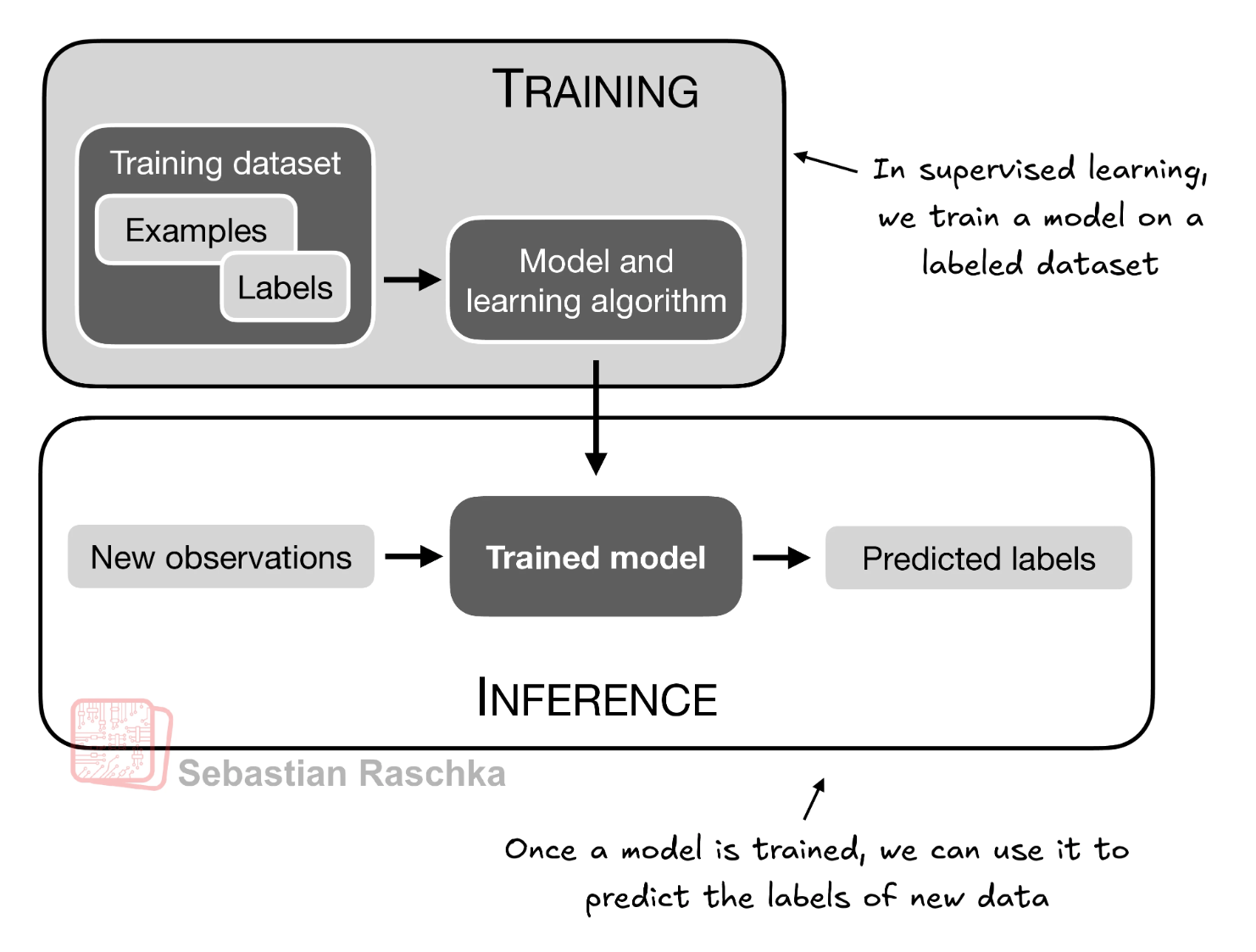
The Training Workflow:

1. Training: A model learns from a labeled dataset (examples + labels).
2. Inference: The trained model predicts labels for new, unseen observations.

1.3 Installing PyTorch

PyTorch offers different versions for CPU and GPU (CUDA).

• If you have a compatible NVIDIA GPU (e.g., RTX 2080 Ti, T4, A100), install the GPU version for significantly faster training.

• For Apple Mac users with M1/M2/M3 chips, PyTorch supports acceleration via MPS (Metal Performance Shaders).

import torch
import sys

# 1. Check PyTorch Version
# The tutorial recommends PyTorch 2.4.1 for compatibility
print(f"PyTorch version: {torch.__version__}")
print(f"Python version: {sys.version}")

# 2. Check for GPU Availability
if torch.cuda.is_available():
    print(f"CUDA (NVIDIA GPU) available: True")
    print(f"Device Name: {torch.cuda.get_device_name(0)}")
    device = torch.device("cuda")
elif torch.backends.mps.is_available():
    print("Apple Silicon (MPS) available: True")
    device = torch.device("mps")
else:
    print("GPU not available. Using CPU.")
    device = torch.device("cpu")

---

2. Understanding Tensors

Tensors are the fundamental building blocks in PyTorch. They are data containers that generalize vectors and matrices to arbitrary dimensions (ranks).

Why Tensors Matter:

• They represent all data in PyTorch: images, text, audio, and model parameters
• They support GPU acceleration for faster computation
• They integrate seamlessly with automatic differentiation for backpropagation

2.1 Scalars, Vectors, Matrices, and Tensors

Scalar (Rank 0): A single number (0-dimensional).

• Example: Temperature reading (72.5°F), a single prediction value
• Shape: ()
• Use case: Loss values, learning rates, individual predictions

Vector (Rank 1): A 1D array of numbers.

• Example: Features of a single data point [age, height, weight]
• Shape: (n,) where n is the number of elements
• Use case: Word embeddings, flattened images, feature vectors

Matrix (Rank 2): A 2D array with rows and columns.

• Example: A grayscale image (height × width), a batch of feature vectors
• Shape: (m, n) where m = rows, n = columns
• Use case: Weight matrices in neural networks, single-channel images, tabular data

3D Tensor (Rank 3): A stack of matrices

• Example: RGB image (height × width × 3 channels), a sequence of feature vectors
• Shape: (d1, d2, d3)
• Use case: Color images, video frames, time series data with multiple features

4D Tensor (Rank 4): Common in deep learning

• Example: A batch of RGB images (batch_size × channels × height × width)
• Shape: (batch_size, channels, height, width)
• Use case: Mini-batches of images for CNNs

Higher Dimensions: Less common but used in specialized applications

• 5D: Video batches (batch × time × channels × height × width)
• 6D and beyond: Rare, used in specialized scientific applications

# Create a 0D tensor (Scalar)
tensor0d = torch.tensor(1)
print(f"Scalar: {tensor0d}, Rank: {tensor0d.ndim}")

# Create a 1D tensor (Vector)
tensor1d = torch.tensor([1, 2, 3])
print(f"Vector: {tensor1d}, Rank: {tensor1d.ndim}")

# Create a 2D tensor (Matrix)
tensor2d = torch.tensor([[1, 2], [3, 4]])
print(f"Matrix shape: {tensor2d.shape}, Rank: {tensor2d.ndim}")

# Create a 3D tensor
tensor3d = torch.tensor([[[1, 2], [3, 4]], [[5, 6], [7, 8]]])
print(f"3D Tensor shape: {tensor3d.shape}, Rank: {tensor3d.ndim}")

2.2 Tensor Data Types and Memory Requirements

PyTorch tensors have specific data types (dtype) that determine precision and memory usage. Understanding these is crucial for optimizing model performance and memory efficiency.

Common PyTorch Data Types:

Integer Types:

• torch.int8 (1 byte per element): Range [-128, 127] - Used for quantized models
• torch.int16 (2 bytes): Range [-32,768, 32,767]
• torch.int32 (4 bytes): Range ±2.1 billion
• torch.int64 (8 bytes): Range ±9.2 quintillion - Default for integers

Floating Point Types:

• torch.float16 (2 bytes): Half precision - Limited range, fast on modern GPUs
• torch.float32 (4 bytes): Single precision - Default for deep learning - Good balance of precision and speed
• torch.float64 (8 bytes): Double precision - High precision but slower, rarely needed in deep learning

Boolean Type:

• torch.bool (1 byte): True/False values - Used for masks and conditions

Complex Types:

• torch.complex64 (8 bytes): For complex number computations
• torch.complex128 (16 bytes): Double precision complex numbers

Memory Calculations:

Example 1: RGB Image (224×224 pixels, 3 channels)

• float32 dtype: 224 × 224 × 3 × 4 bytes = 602,112 bytes ≈ 0.6 MB
• float16 dtype: 224 × 224 × 3 × 2 bytes = 301,056 bytes ≈ 0.3 MB (50% savings!)

Example 2: ResNet-50 Model Parameters (~25.5 million parameters)

• float32: 25,500,000 × 4 bytes = 102 MB
• float16: 25,500,000 × 2 bytes = 51 MB

Example 3: Batch of 32 Images (224×224×3)

• float32: 32 × 224 × 224 × 3 × 4 = 19.3 MB per batch

When to Use Each Type:

• float32 (most common): Default for training neural networks - provides sufficient precision for gradients
• float16 (mixed precision training): Use with automatic mixed precision (AMP) to speed up training on modern GPUs (V100, A100, RTX series)
• float64: Scientific computing requiring high precision, rarely needed in deep learning
• int64: Labels, indices, discrete data
• int8: Model quantization for deployment on edge devices (reduces model size by 75%)

Memory Tip: Using float16 can allow you to double your batch size, leading to faster training!

# Default integer type (int64)
t_int = torch.tensor([1, 2, 3])
print(f"Integer Tensor Type: {t_int.dtype}")
print(f"Memory per element: {t_int.element_size()} bytes")
print(f"Total memory: {t_int.numel() * t_int.element_size()} bytes\n")

# Default float type (float32) - Created by using dots in numbers
t_float = torch.tensor([1., 2., 3.])
print(f"Float Tensor Type: {t_float.dtype}")
print(f"Memory per element: {t_float.element_size()} bytes")
print(f"Total memory: {t_float.numel() * t_float.element_size()} bytes\n")

# Explicitly specifying data type (float64)
t_explicit = torch.tensor([1, 2, 3], dtype=torch.float64)
print(f"Explicit Type: {t_explicit.dtype}")
print(f"Memory per element: {t_explicit.element_size()} bytes")
print(f"Total memory: {t_explicit.numel() * t_explicit.element_size()} bytes\n")

# Float16 for memory efficiency
t_half = torch.tensor([1., 2., 3.], dtype=torch.float16)
print(f"Half Precision Type: {t_half.dtype}")
print(f"Memory per element: {t_half.element_size()} bytes")
print(f"Total memory: {t_half.numel() * t_half.element_size()} bytes (50% savings!)")

# Demonstrate memory difference with a larger tensor
large_tensor_f32 = torch.randn(1000, 1000, dtype=torch.float32)
large_tensor_f16 = torch.randn(1000, 1000, dtype=torch.float16)
print(f"\n1000x1000 tensor in float32: {large_tensor_f32.element_size() * large_tensor_f32.numel() / (1024**2):.2f} MB")
print(f"1000x1000 tensor in float16: {large_tensor_f16.element_size() * large_tensor_f16.numel() / (1024**2):.2f} MB")

2.3 Common PyTorch Tensor Operations

PyTorch adopts a syntax very similar to NumPy for mathematical operations. These operations are the building blocks of neural networks.

Key Operations:

1. Element-wise Operations: Apply operation to each element independently

• Addition, subtraction, multiplication, division
• Tensors must have compatible shapes (broadcasting rules apply)

2. Matrix Multiplication (matmul): The heart of neural networks

• Forward pass: outputs = weights @ inputs
• Essential for computing layer activations
• Use @ operator or torch.matmul()

3. Reshaping Operations: Change tensor dimensions without changing data

• view(): Creates a new view (shares memory)
• reshape(): More flexible, may copy data
• -1 in shape means “infer this dimension”
• Common use: Flatten images for fully connected layers

4. Aggregation Operations: Reduce dimensions

• sum(), mean(), max(), min(): Compute statistics
• Specify dim parameter to aggregate along specific dimension

5. Indexing and Slicing: Access tensor elements

• Similar to NumPy: tensor[0, :, 1:3]
• Boolean indexing: tensor[tensor > 0]

# Creation
x = torch.tensor([[1, 2], [3, 4]], dtype=torch.float32)
y = torch.tensor([[5, 6], [7, 8]], dtype=torch.float32)

# Element-wise addition (each element paired with corresponding element)
print("Addition:\n", x + y)
print("Also works:", torch.add(x, y))

# Element-wise multiplication (NOT matrix multiplication!)
print("\nElement-wise multiplication:\n", x * y)

# Matrix Multiplication (matmul) - CRUCIAL for Neural Networks
# Rule: (m x n) @ (n x p) = (m x p)
# Here: (2x2) @ (2x2) = (2x2)
print("\nMatrix Multiplication (Weights * Inputs):\n", x @ y) # OR torch.matmul(x, y)

# Reshaping - Common when flattening images (e.g., 28x28 -> 784 vector)
print("\nOriginal shape:", x.shape)
flat = x.view(-1)  # -1 means "infer this dimension"
print("Flattened to 1D:", flat, "Shape:", flat.shape)

# Reshape to different configuration
reshaped = x.view(4, 1)
print("\nReshaped to column vector:\n", reshaped, "Shape:", reshaped.shape)

# Aggregation operations
print("\nSum of all elements:", x.sum())
print("Mean:", x.mean())
print("Max:", x.max())
print("Sum along rows (dim=0):", x.sum(dim=0))  # Sum each column
print("Sum along columns (dim=1):", x.sum(dim=1))  # Sum each row

# Broadcasting - automatically expand dimensions to match
a = torch.tensor([1, 2, 3])
b = torch.tensor([[1], [2]])
print("\nBroadcasting:")
print("a shape:", a.shape, "b shape:", b.shape)
print("a + b (broadcasted):\n", a + b)  # (2,3) result

---

3. Seeing Models as Computation Graphs

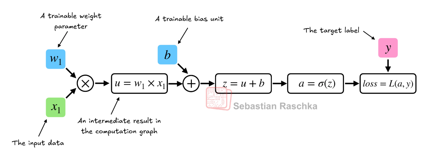
Deep learning models are essentially computation graphs - a series of mathematical operations where each operation is a node, and the edges represent data flow.

Why Computation Graphs Matter:

1. Automatic Differentiation: PyTorch tracks all operations to compute gradients automatically
2. Optimization: The graph structure allows PyTorch to optimize memory usage and execution
3. Debugging: Understanding the graph helps debug gradient flow issues

3.1 Simple Perceptron Example

In a simple neuron (perceptron), the computation flow is:

1. Input (x) multiplied by Weight (w): $u = w \times x$
2. Add Bias (b): $z = u + b$
3. Apply Activation (σ): $a = \sigma(z)$ (e.g., sigmoid, ReLU)
4. Compute Loss (L) against target (y): $L = (a - y)^2$ (Mean Squared Error)

How PyTorch Builds the Graph:

• Each operation creates a new node in the graph
• PyTorch stores the history of operations for tensors with requires_grad=True
• During .backward(), PyTorch traverses the graph in reverse to compute gradients

Graph Properties:

• Forward Pass: Data flows from inputs to outputs (left to right)
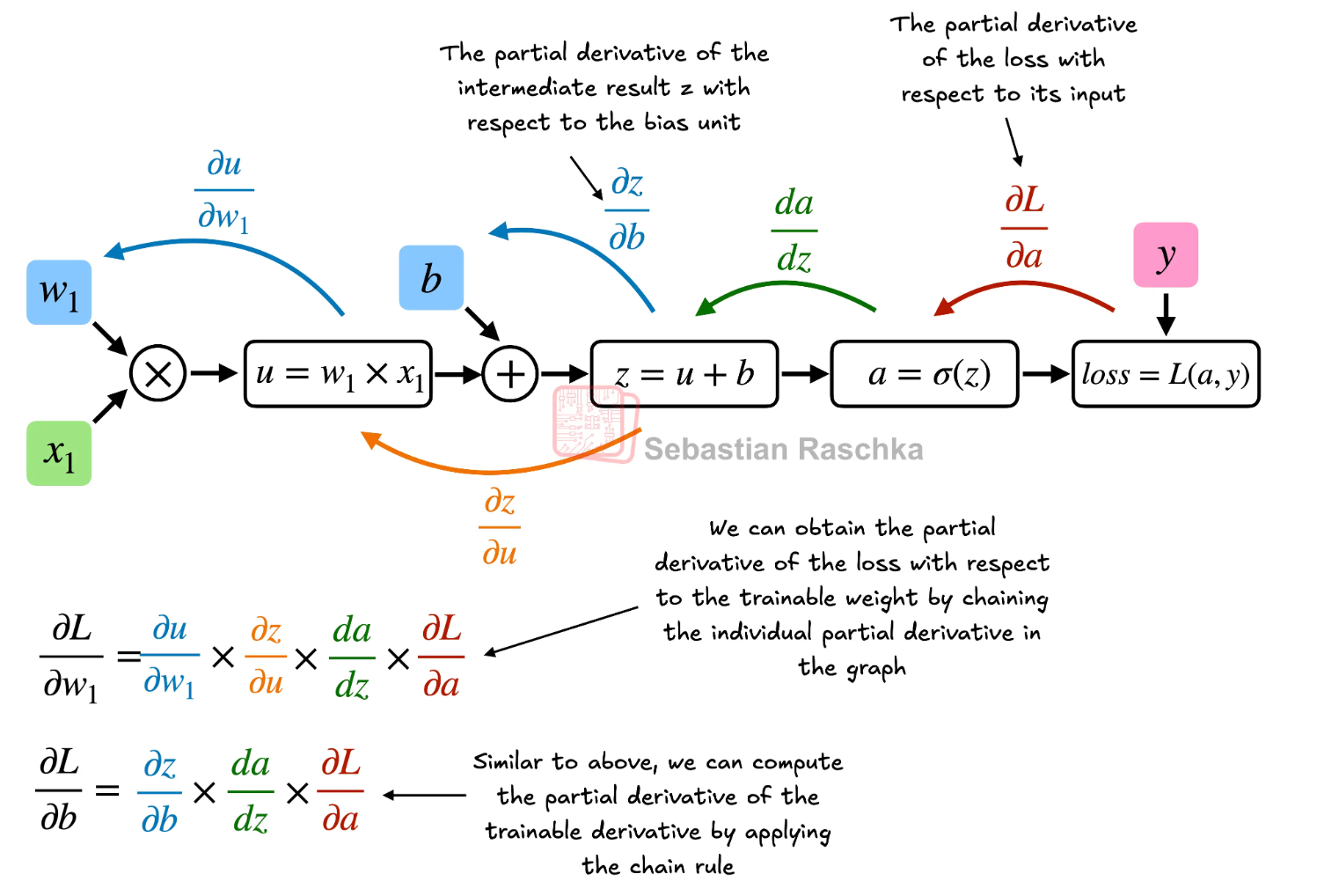
• Backward Pass: Gradients flow from loss to parameters (right to left)
• Dynamic Computation Graph: PyTorch builds the graph on-the-fly (define-by-run), allowing for flexible architectures

3.2 Memory Considerations

Each operation in the graph stores intermediate values for gradient computation:

• Forward pass memory: Stores activations for each layer
• Backward pass memory: Stores gradients for each parameter
• Total memory = model parameters + activations + gradients + optimizer states

For a simple layer with input size 1000 and output size 500:

• Parameters: 1000 × 500 = 500,000 weights (2 MB in float32)
• Activations: Depends on batch size (e.g., batch=32: 32 × 500 = 16,000 values = 64 KB)
• Gradients: Same size as parameters (2 MB)

---

4. Automatic Differentiation Made Easy

PyTorch’s autograd engine computes gradients automatically. This is essential for backpropagation, where we update weights to minimize loss.

The Chain Rule in Action:

We calculate partial derivatives (gradients) of the loss with respect to weights: $\frac{\partial L}{\partial w}$

For a computation chain: $x \rightarrow u \rightarrow z \rightarrow a \rightarrow L$

Using the chain rule: $\frac{\partial L}{\partial w} = \frac{\partial L}{\partial a} \times \frac{\partial a}{\partial z} \times \frac{\partial z}{\partial u} \times \frac{\partial u}{\partial w}$

PyTorch does this automatically!

4.1 How Autograd Works

1. Forward Pass: Compute outputs and build the computation graph
2. Backward Pass: Call .backward() to compute gradients using chain rule
3. Access Gradients: Read .grad attribute of tensors
4. Update Parameters: Use gradients to adjust weights (done by optimizer)

Important Notes:

• Only tensors with requires_grad=True participate in gradient computation
• Gradients accumulate by default - use optimizer.zero_grad() to clear them
• .backward() can only be called once on non-leaf nodes (unless retain_graph=True)
• For scalar loss, no argument needed; for vector, must specify gradient parameter

# Initialize tensors with gradients enabled
# 'requires_grad=True' tells PyTorch to build the computation graph for these tensors
w = torch.tensor([1.0], requires_grad=True)
b = torch.tensor([0.5], requires_grad=True)
x = torch.tensor([1.0])  # Inputs usually do not require gradients
y_target = torch.tensor([2.0])

print("Initial Parameters:")
print(f"Weight (w): {w.item():.4f}")
print(f"Bias (b): {b.item():.4f}\n")

# 1. Forward Pass (Building the computation graph)
# Each operation creates a node in the graph
u = w * x          # Node 1: Multiplication
z = u + b          # Node 2: Addition
a = torch.sigmoid(z) # Node 3: Activation function
loss = (a - y_target)**2 # Node 4: Mean Squared Error loss

print("Forward Pass Results:")
print(f"u = w * x = {u.item():.4f}")
print(f"z = u + b = {z.item():.4f}")
print(f"a = sigmoid(z) = {a.item():.4f}")
print(f"Loss = (a - y_target)² = {loss.item():.4f}\n")

# 2. Backward Pass (Automatic Differentiation)
# This computes dLoss/dw and dLoss/db using the chain rule
# PyTorch traverses the graph backwards from loss to parameters
loss.backward()

# 3. Check Gradients
print("Computed Gradients (How much to change each parameter):")
print(f"Gradient dL/dw: {w.grad.item():.6f}")
print(f"Gradient dL/db: {b.grad.item():.6f}\n")

# These gradients tell us:
# - Positive gradient: Increasing the parameter increases the loss (move in negative direction)
# - Negative gradient: Increasing the parameter decreases the loss (move in positive direction)
# - Magnitude: How sensitive the loss is to changes in this parameter

print("Interpretation:")
if w.grad.item() > 0:
    print(f"→ Weight gradient is positive: Decrease w to reduce loss")
else:
    print(f"→ Weight gradient is negative: Increase w to reduce loss")
    
if b.grad.item() > 0:
    print(f"→ Bias gradient is positive: Decrease b to reduce loss")
else:
    print(f"→ Bias gradient is negative: Increase b to reduce loss")

# Example of parameter update (done automatically by optimizers)
learning_rate = 0.1
print(f"\nManual Parameter Update (learning_rate={learning_rate}):")
print(f"New w = {w.item():.4f} - {learning_rate} * {w.grad.item():.6f} = {w.item() - learning_rate * w.grad.item():.4f}")
print(f"New b = {b.item():.4f} - {learning_rate} * {b.grad.item():.6f} = {b.item() - learning_rate * b.grad.item():.4f}")

---

5. Implementing Multilayer Neural Networks

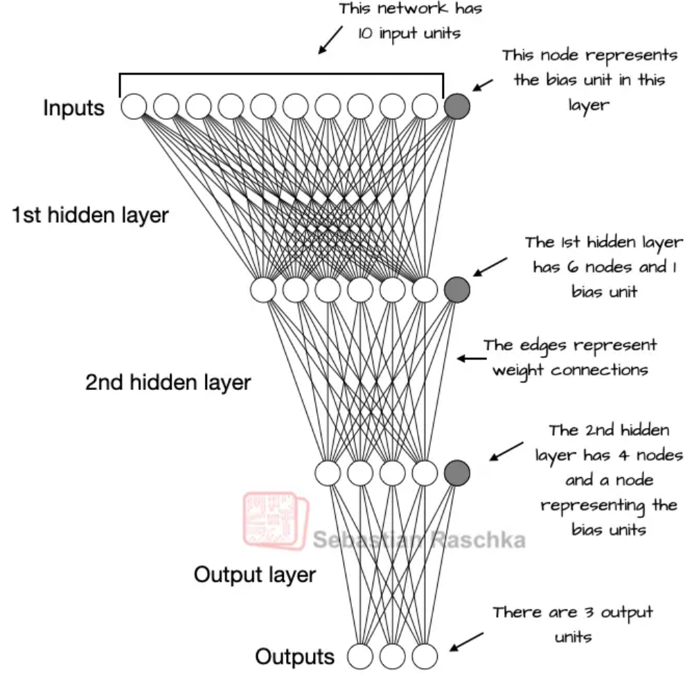
A deep neural network consists of multiple layers of neurons stacked together. We define these using torch.nn, which provides pre-built, optimized layers.

5.1 Network Architecture

The structure typically involves:

• Input Layer: Receives the raw data features (not explicitly defined in PyTorch)

  • Size = number of features in your data
  • Example: 784 for flattened 28×28 MNIST images

• Hidden Layers: Learn complex, nonlinear representations

  • Multiple hidden layers = “deep” network
  • Each layer transforms data into increasingly abstract features
  • Activation functions (ReLU, Tanh, etc.) add non-linearity

• Output Layer: Produces the final prediction

  • Size depends on task:
    • Binary classification: 1 unit (with sigmoid) or 2 units (with softmax)
    • Multi-class: number of classes (e.g., 10 for digit recognition)
    • Regression: 1 or more (number of values to predict)

5.2 Understanding Layer Dimensions

Linear Layer (Fully Connected):

• Formula: output = input @ weight.T + bias
• Parameters: input_dim × output_dim weights + output_dim biases
• Example: nn.Linear(10, 5) has 10 × 5 = 50 weights + 5 biases = 55 parameters

Parameter Counting Example:

• Layer 1: Linear(784, 128) → 784 × 128 + 128 = 100,480 parameters
• Layer 2: Linear(128, 64) → 128 × 64 + 64 = 8,256 parameters
• Layer 3: Linear(64, 10) → 64 × 10 + 10 = 650 parameters
• Total: 109,386 parameters

In float32: 109,386 × 4 bytes = 437.5 KB (just the model parameters!)

5.3 Activation Functions

Why we need them: Without activation functions, multiple linear layers collapse into a single linear transformation (no benefit from depth)

Common Choices:

• ReLU (max(0, x)): Most popular, fast, helps with vanishing gradients
• Sigmoid (1 / (1 + e^-x)): Outputs [0,1], used for probabilities
• Tanh ((e^x - e^-x) / (e^x + e^-x)): Outputs [-1,1], zero-centered
• Softmax: Converts logits to probability distribution (sum=1)

import torch.nn as nn

class MultilayerPerceptron(nn.Module):
    def __init__(self, input_dim, hidden_dim, output_dim):
        super().__init__()
        # First hidden layer (Linear transformation)
        # Parameters: input_dim × hidden_dim weights + hidden_dim biases
        self.layer1 = nn.Linear(input_dim, hidden_dim)
        
        # Non-linear activation function (ReLU)
        # No learnable parameters - just applies max(0, x)
        self.relu = nn.ReLU()
        
        # Output layer
        # Parameters: hidden_dim × output_dim weights + output_dim biases
        self.layer2 = nn.Linear(hidden_dim, output_dim)

    def forward(self, x):
        # Define the flow of data through the network
        # Input shape: (batch_size, input_dim)
        x = self.layer1(x)  # Shape: (batch_size, hidden_dim)
        x = self.relu(x)    # Shape: (batch_size, hidden_dim) - no change
        x = self.layer2(x)  # Shape: (batch_size, output_dim)
        return x

# Instantiate the model
# Example: 10 input features, 5 hidden units, 1 output unit (e.g., binary classification)
model = MultilayerPerceptron(input_dim=10, hidden_dim=5, output_dim=1)
print(model)
print("\n" + "="*60)

# Count parameters
total_params = sum(p.numel() for p in model.parameters())
trainable_params = sum(p.numel() for p in model.parameters() if p.requires_grad)

print(f"\nModel Architecture Summary:")
print(f"Total parameters: {total_params:,}")
print(f"Trainable parameters: {trainable_params:,}")

# Breakdown by layer
print("\nDetailed Parameter Count:")
for name, param in model.named_parameters():
    print(f"{name:20s}: {param.numel():6,} parameters, Shape: {list(param.shape)}")

# Calculate memory usage
memory_bytes = total_params * 4  # float32 = 4 bytes per parameter
print(f"\nMemory Usage (float32): {memory_bytes:,} bytes = {memory_bytes/1024:.2f} KB")

# Test with sample input
print("\n" + "="*60)
print("Testing forward pass:")
sample_input = torch.randn(3, 10)  # Batch of 3 samples, each with 10 features
print(f"Input shape: {sample_input.shape}")
output = model(sample_input)
print(f"Output shape: {output.shape}")
print(f"Output values:\n{output}")

---

6. Setting up Efficient Data Loaders

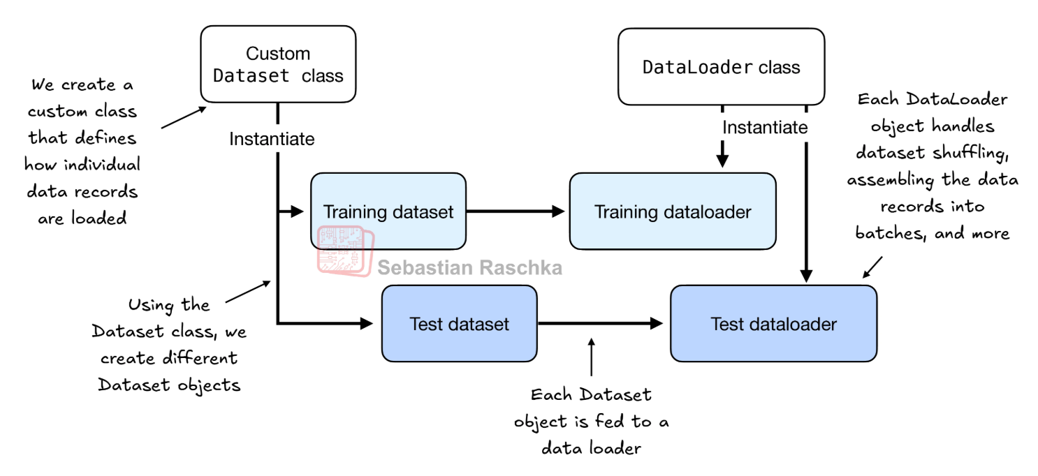Manually loading data can create bottlenecks and slow down training. PyTorch uses Dataset and DataLoader classes to handle data efficiently with minimal overhead.

6.1 Key Components

• Dataset: Stores samples and labels

  • Implements __len__() (returns dataset size)
  • Implements __getitem__() (returns one sample)
  • Can be custom (load from disk) or built-in (TensorDataset for in-memory data)

• DataLoader: Iterates through the dataset intelligently

  • Creates mini-batches (small groups of data)
  • Shuffles data (breaks correlations between consecutive samples)
  • Handles multi-threaded data loading (parallel workers)
  • Automatically handles padding and collation

6.2 Batch Size Considerations

What is Batch Size? The number of samples processed together before updating model parameters.

Trade-offs:

• Large batches (128, 256, 512):

  • ✅ More stable gradients (smoother training)
  • ✅ Better GPU utilization (parallel processing)
  • ✅ Faster training per epoch
  • ❌ Requires more memory
  • ❌ May lead to poorer generalization

• Small batches (16, 32, 64):

  • ✅ Less memory required
  • ✅ More frequent weight updates
  • ✅ Often better generalization
  • ❌ Noisier gradients
  • ❌ Slower training per epoch

Memory Formula: Memory per batch ≈ batch_size × model_input_size × 4 bytes (float32)

Example: Batch of 32 images (224×224×3):

• 32 × 224 × 224 × 3 × 4 bytes = 19.3 MB

Rule of Thumb: Start with batch size 32 or 64, increase until GPU memory is ~80% full

6.3 Data Loading Best Practices

1. Shuffle Training Data: shuffle=True prevents the model from learning order patterns
2. Don’t Shuffle Validation/Test: Keep evaluation consistent
3. Use Multiple Workers: num_workers=4 for parallel data loading (CPU-bound tasks)
4. Pin Memory: pin_memory=True speeds up CPU-to-GPU transfer

from torch.utils.data import DataLoader, TensorDataset

# Create dummy dataset (100 samples, 10 features each)
X = torch.randn(100, 10)
y = torch.randn(100, 1)

print(f"Dataset size: {X.shape[0]} samples")
print(f"Feature dimension: {X.shape[1]}")
print(f"Target dimension: {y.shape[1]}\n")

dataset = TensorDataset(X, y)

# Create DataLoader with common settings
# shuffle=True: Randomly reorder data each epoch (prevents learning order patterns)
# batch_size: Number of samples per batch
loader = DataLoader(dataset, batch_size=32, shuffle=True)

print(f"DataLoader created:")
print(f"  Batch size: {loader.batch_size}")
print(f"  Shuffle: {loader._dataset_kind == 0}")  # Internal check
print(f"  Number of batches: {len(loader)}")  # 100 samples / 32 per batch = 4 batches
print(f"  Last batch size: {100 % 32} (remainder)\n")

# Inspect one batch
X_batch, y_batch = next(iter(loader))
print(f"Single Batch Shapes:")
print(f"  X_batch: {X_batch.shape} (batch_size, features)")
print(f"  y_batch: {y_batch.shape} (batch_size, targets)\n")

# Calculate memory per batch
memory_per_batch = X_batch.numel() * X_batch.element_size() + y_batch.numel() * y_batch.element_size()
print(f"Memory per batch: {memory_per_batch:,} bytes = {memory_per_batch/1024:.2f} KB\n")

# Show how batches iterate
print("Iterating through batches:")
for i, (batch_x, batch_y) in enumerate(loader):
    print(f"  Batch {i+1}: X={batch_x.shape}, y={batch_y.shape}")
    
print("\n" + "="*60)
print("Effect of Different Batch Sizes:")
for bs in [16, 32, 64, 128]:
    if bs <= len(dataset):
        temp_loader = DataLoader(dataset, batch_size=bs)
        print(f"  Batch size {bs:3d}: {len(temp_loader)} batches, last batch has {len(dataset) % bs if len(dataset) % bs > 0 else bs} samples")

---

7. A Typical Training Loop

A standard PyTorch training loop iterates over the dataset (epochs) and processes batches. For each batch, it performs 5 distinct steps:

7.1 The Five Steps Explained

1. Forward Pass: Compute model predictions

   • Pass input data through the network
   • Get output predictions
   • Shape: (batch_size, output_dim)

2. Compute Loss: Calculate how wrong the model is

   • Compare predictions with ground truth labels
   • Common losses: MSE (regression), CrossEntropy (classification)
   • Returns a scalar value

3. Zero Gradients: Clear old gradients from the previous step

   • Gradients accumulate by default in PyTorch
   • Must call optimizer.zero_grad() before each backward pass
   • Otherwise, gradients from previous batches are added to current gradients

4. Backward Pass: Compute new gradients using loss.backward()

   • Automatically computes ∂Loss/∂parameter for all parameters
   • Uses chain rule to propagate gradients backwards
   • Stores gradients in .grad attribute of each parameter

5. Optimization Step: Update weights using optimizer.step()

   • Applies gradient descent: parameter = parameter - learning_rate × gradient
   • Different optimizers use different update rules (SGD, Adam, etc.)

7.2 Key Concepts

Epoch: One complete pass through the entire training dataset

• Example: 1000 samples with batch_size=100 → 10 batches per epoch

Learning Rate: Controls step size for parameter updates

• Too high: Training unstable, loss explodes
• Too low: Training very slow, may get stuck
• Typical values: 0.001, 0.0001 for Adam; 0.01, 0.1 for SGD

Loss Function Selection:

• Regression: MSELoss, L1Loss, SmoothL1Loss
• Binary Classification: BCELoss (with sigmoid), BCEWithLogitsLoss
• Multi-class Classification: CrossEntropyLoss (includes softmax)

Optimizer Selection:

• SGD: Simple, requires careful learning rate tuning
• Adam: Adaptive learning rate, most popular, works well out-of-the-box
• AdamW: Adam with better weight decay (current best practice)

7.3 Monitoring Training

Track these metrics:

• Training Loss: Should decrease over time
• Validation Loss: Should decrease; if it increases → overfitting
• Training Time: Monitor to optimize efficiency
• GPU Memory Usage: Adjust batch size if needed

import torch.optim as optim
import time

# Setup
learning_rate = 0.01
criterion = nn.MSELoss() # Loss function (Mean Squared Error for regression)
optimizer = optim.SGD(model.parameters(), lr=learning_rate) # Stochastic Gradient Descent

print("Training Configuration:")
print(f"  Optimizer: SGD")
print(f"  Learning Rate: {learning_rate}")
print(f"  Loss Function: MSE")
print(f"  Epochs: 5")
print(f"  Batch Size: {loader.batch_size}")
print(f"  Number of Batches per Epoch: {len(loader)}\n")
print("="*60)

# Training Loop
epochs = 5
for epoch in range(epochs):
    running_loss = 0.0
    epoch_start_time = time.time()

    # Iterate through all batches in the dataset
    for i, (inputs, targets) in enumerate(loader):
        # Step 1: Forward pass
        # Pass inputs through the model to get predictions
        outputs = model(inputs)

        # Step 2: Compute loss
        # Calculate how far predictions are from targets
        loss = criterion(outputs, targets)

        # Step 3: Zero gradients
        # Clear gradients from previous iteration (they accumulate by default)
        optimizer.zero_grad()

        # Step 4: Backward pass
        # Compute gradients of loss w.r.t. all parameters
        # Uses automatic differentiation (autograd)
        loss.backward()

        # Step 5: Update weights
        # Apply gradient descent: θ = θ - lr * ∇θ
        optimizer.step()

        # Accumulate loss for monitoring
        running_loss += loss.item()

    # Calculate statistics for this epoch
    epoch_time = time.time() - epoch_start_time
    avg_loss = running_loss / len(loader)
    
    print(f"Epoch {epoch+1}/{epochs}:")
    print(f"  Average Loss: {avg_loss:.4f}")
    print(f"  Total Loss: {running_loss:.4f}")
    print(f"  Time: {epoch_time:.2f}s")
    print(f"  Batches Processed: {len(loader)}")
    
    # Show sample prediction from last batch
    if epoch == epochs - 1:
        print(f"\n  Sample predictions from last batch:")
        print(f"    First 3 predictions: {outputs[:3].detach().squeeze().numpy()}")
        print(f"    First 3 targets:     {targets[:3].squeeze().numpy()}")

print("\n" + "="*60)
print("Training completed!")
print(f"Final Average Loss: {avg_loss:.4f}")

---

8. Saving and Loading Models

Deep learning models can take hours or days to train. It is essential to save model parameters (weights and biases) to avoid retraining.

8.1 Two Approaches to Saving

1. Save State Dict (Recommended):

• Saves only the parameters (weights and biases)
• More flexible - can load into different code versions
• Smaller file size
• Use: torch.save(model.state_dict(), 'model.pth')

2. Save Entire Model:

• Saves model architecture + parameters
• Less flexible - tied to specific code structure
• Use: torch.save(model, 'model.pth')

8.2 Best Practices

What to Save:

• Model state dict: model.state_dict()
• Optimizer state dict: optimizer.state_dict() (for resuming training)
• Epoch number: Current epoch (for resuming)
• Loss history: Track training progress

File Formats:

• .pth or .pt: PyTorch convention
• Files are actually pickled Python objects

Loading Requirements:

• Must define the model architecture before loading
• Architecture must match exactly (same layer sizes)
• Use model.eval() before inference (disables dropout, batch norm training mode)

8.3 Modes: Training vs Evaluation

Training Mode (model.train()):

• Dropout is active (randomly drops neurons)
• Batch normalization uses batch statistics
• Gradients are computed

Evaluation Mode (model.eval()):

• Dropout is disabled (all neurons active)
• Batch normalization uses running statistics
• Use with torch.no_grad() to save memory (no gradient computation)

# Saving the model parameters (state_dict) - RECOMMENDED METHOD
checkpoint_path = "my_model.pth"
torch.save(model.state_dict(), checkpoint_path)
print(f"✓ Model saved to {checkpoint_path}")

# Check file size
import os
file_size = os.path.getsize(checkpoint_path)
print(f"  File size: {file_size:,} bytes = {file_size/1024:.2f} KB\n")

# Loading the model
loaded_model = MultilayerPerceptron(10, 5, 1) # Must match original architecture!
loaded_model.load_state_dict(torch.load(checkpoint_path))
loaded_model.eval() # Set to evaluation mode (important for inference)
print("✓ Model loaded successfully!")
print(f"  Model is in {'training' if loaded_model.training else 'evaluation'} mode\n")

# Verify the models are identical
print("Verification: Comparing original vs loaded model")
original_params = list(model.parameters())
loaded_params = list(loaded_model.parameters())

all_match = True
for i, (orig, load) in enumerate(zip(original_params, loaded_params)):
    match = torch.allclose(orig, load)
    all_match = all_match and match
    print(f"  Parameter {i+1}: {'✓ Match' if match else '✗ Mismatch'}")

print(f"\n{'✓' if all_match else '✗'} Overall: Models are {'identical' if all_match else 'different'}\n")

# Saving a complete training checkpoint (for resuming training)
checkpoint = {
    'epoch': 5,
    'model_state_dict': model.state_dict(),
    'optimizer_state_dict': optimizer.state_dict(),
    'loss': avg_loss,
}
torch.save(checkpoint, 'checkpoint.pth')
print("✓ Training checkpoint saved (includes optimizer state)")

# Loading a checkpoint to resume training
checkpoint = torch.load('checkpoint.pth')
model.load_state_dict(checkpoint['model_state_dict'])
optimizer.load_state_dict(checkpoint['optimizer_state_dict'])
epoch = checkpoint['epoch']
loss = checkpoint['loss']
print(f"✓ Checkpoint loaded: Epoch {epoch}, Loss {loss:.4f}")

# Making predictions with loaded model
print("\nTesting loaded model with sample input:")
model.eval()
with torch.no_grad():  # Disable gradient computation for inference (saves memory)
    test_input = torch.randn(2, 10)
    predictions = model(test_input)
    print(f"  Input shape: {test_input.shape}")
    print(f"  Predictions: {predictions.squeeze().numpy()}")

---

8.5 Model Complexity Analysis: Counting FLOPs

FLOPs (Floating Point Operations) measure the computational complexity of a neural network. Understanding FLOPs helps you:

• Compare model efficiency
• Estimate inference speed
• Optimize for deployment on resource-constrained devices
• Choose between model architectures

8.5.1 What are FLOPs?

FLOP: One floating-point operation (addition, multiplication, etc.) FLOPs: Total number of operations for one forward pass FLOPS (with ‘S’): FLOPs Per Second (throughput metric)

Common Operations:

• Linear Layer: 2 × input_dim × output_dim × batch_size FLOPs
  • Factor of 2: multiply-accumulate counts as 2 ops (multiply + add)
• Convolution: 2 × C_in × C_out × K_h × K_w × H_out × W_out × batch_size
• Activation (ReLU): 1 × num_elements FLOPs (very cheap)

8.5.2 FLOPs vs Parameters

These are different metrics:

• Parameters: Memory footprint (storage size)
• FLOPs: Computational cost (inference speed)

Example: MobileNet vs ResNet-50

• MobileNet: 4.2M params, 0.6 GFLOPs - Fast, small
• ResNet-50: 25.6M params, 4.1 GFLOPs - Slower, larger

8.5.3 Calculating FLOPs

We’ll use the fvcore library (from Facebook Research) for accurate FLOP counting:

pip install fvcore

Alternatively, use thop (THe OPeration counter):

pip install thop

Method 1: Manual FLOP Calculation

# Method 1: Manual FLOP Calculation for our MLP
print("="*60)
print("Method 1: Manual FLOP Calculation")
print("="*60)

# Our model: Linear(10, 5) -> ReLU -> Linear(5, 1)
input_dim = 10
hidden_dim = 5
output_dim = 1
batch_size = 1  # For single inference

# Layer 1: Linear(10, 5)
# Formula: 2 * input_dim * output_dim (multiply-accumulate for each output neuron)
flops_layer1 = 2 * input_dim * hidden_dim
print(f"\nLayer 1 [Linear(10, 5)]:")
print(f"  FLOPs = 2 × {input_dim} × {hidden_dim} = {flops_layer1:,}")

# ReLU activation
flops_relu = hidden_dim  # One comparison per element
print(f"\nReLU Activation:")
print(f"  FLOPs = {hidden_dim} (very cheap)")

# Layer 2: Linear(5, 1)
flops_layer2 = 2 * hidden_dim * output_dim
print(f"\nLayer 2 [Linear(5, 1)]:")
print(f"  FLOPs = 2 × {hidden_dim} × {output_dim} = {flops_layer2:,}")

# Total FLOPs
total_flops_manual = flops_layer1 + flops_relu + flops_layer2
print(f"\n{'='*60}")
print(f"Total FLOPs per inference: {total_flops_manual:,}")
print(f"Total FLOPs in millions (MFLOPs): {total_flops_manual / 1e6:.4f}")
print(f"Total FLOPs in billions (GFLOPs): {total_flops_manual / 1e9:.6f}")

# For a batch
batch_size = 32
batch_flops = total_flops_manual * batch_size
print(f"\nFor batch size {batch_size}:")
print(f"  Total FLOPs: {batch_flops:,}")
print(f"  GFLOPs: {batch_flops / 1e9:.6f}")

Method 2: Using thop Library

# Method 2: Using thop library (if available)
print("\n" + "="*60)
print("Method 2: Using thop Library")
print("="*60)

try:
    from thop import profile, clever_format
    
    # Create a fresh model instance
    model_for_flops = MultilayerPerceptron(input_dim=10, hidden_dim=5, output_dim=1)
    model_for_flops.eval()
    
    # Create sample input
    input_tensor = torch.randn(1, 10)  # Batch size 1
    
    # Profile the model
    flops, params = profile(model_for_flops, inputs=(input_tensor,), verbose=False)
    flops_readable, params_readable = clever_format([flops, params], "%.3f")
    
    print(f"✓ thop library installed and working!")
    print(f"\nResults:")
    print(f"  FLOPs: {flops_readable}")
    print(f"  Parameters: {params_readable}")
    print(f"  Raw FLOPs: {flops:,.0f}")
    print(f"  Raw Parameters: {params:,.0f}")
    
except ImportError:
    print("⚠ thop library not installed")
    print("  Install with: pip install thop")
    print("  This library provides automated FLOP counting")

Method 3: Using fvcore Library

# Method 3: Using fvcore library (if available)
print("\n" + "="*60)
print("Method 3: Using fvcore Library")
print("="*60)

try:
    from fvcore.nn import FlopCountAnalysis, flop_count_table
    
    # Create a fresh model instance
    model_for_fvcore = MultilayerPerceptron(input_dim=10, hidden_dim=5, output_dim=1)
    model_for_fvcore.eval()
    
    # Create sample input
    input_tensor = torch.randn(1, 10)
    
    # Analyze FLOPs
    flops_analysis = FlopCountAnalysis(model_for_fvcore, input_tensor)
    total_flops = flops_analysis.total()
    
    print(f"✓ fvcore library installed and working!")
    print(f"\nResults:")
    print(f"  Total FLOPs: {total_flops:,}")
    print(f"  MFLOPs: {total_flops / 1e6:.4f}")
    print(f"  GFLOPs: {total_flops / 1e9:.6f}")
    
    # Detailed breakdown by layer
    print(f"\nDetailed Breakdown:")
    print(flop_count_table(flops_analysis))
    
except ImportError:
    print("⚠ fvcore library not installed")
    print("  Install with: pip install fvcore")
    print("  This library provides detailed per-layer FLOP analysis")

8.5.4 Real-World Model Comparisons

Let’s compare computational complexity of popular architectures:

Image Classification Models (ImageNet):

Model	Parameters	FLOPs	Top-1 Accuracy	Speed (GPU)
MobileNetV2	3.5M	0.3B	72.0%	Very Fast
EfficientNet-B0	5.3M	0.4B	77.1%	Fast
ResNet-50	25.6M	4.1B	76.2%	Medium
ResNet-101	44.5M	7.8B	77.4%	Slow
EfficientNet-B7	66.0M	37.0B	84.4%	Very Slow

Key Insights:

• Efficiency: MobileNet achieves decent accuracy with 10× fewer FLOPs than ResNet-50
• Accuracy vs Speed: More FLOPs generally means better accuracy but slower inference
• Architecture Matters: EfficientNet achieves better accuracy per FLOP than ResNet

8.5.5 When FLOPs Matter

Critical for:

• Mobile/Edge deployment (limited compute)
• Real-time applications (video processing)
• Large-scale inference (serving millions of requests)
• Energy-constrained devices (IoT, drones)

Less Critical for:

• One-off predictions
• Small-scale research experiments
• When GPU resources are abundant

8.5.6 Optimizing FLOPs

Techniques to Reduce FLOPs:

1. Depthwise Separable Convolutions (MobileNet): 8-9× fewer FLOPs
2. Pruning: Remove unimportant connections (30-50% reduction)
3. Knowledge Distillation: Train smaller model to mimic larger one
4. Neural Architecture Search: Find efficient architectures automatically
5. Quantization: Reduce precision (int8 instead of float32) - reduces both memory and compute

# Practical Example: Compare different model architectures
print("="*60)
print("Comparing Model Architectures")
print("="*60)

# Define different model sizes
configs = [
    {"name": "Tiny", "input": 10, "hidden": 5, "output": 1},
    {"name": "Small", "input": 10, "hidden": 32, "output": 1},
    {"name": "Medium", "input": 10, "hidden": 128, "output": 1},
    {"name": "Large", "input": 10, "hidden": 512, "output": 1},
]

results = []

for config in configs:
    # Create model
    test_model = MultilayerPerceptron(
        config["input"], 
        config["hidden"], 
        config["output"]
    )
    
    # Count parameters
    n_params = sum(p.numel() for p in test_model.parameters())
    
    # Calculate FLOPs manually
    layer1_flops = 2 * config["input"] * config["hidden"]
    relu_flops = config["hidden"]
    layer2_flops = 2 * config["hidden"] * config["output"]
    total_flops = layer1_flops + relu_flops + layer2_flops
    
    # Memory (float32)
    memory_mb = (n_params * 4) / (1024**2)
    
    results.append({
        "name": config["name"],
        "params": n_params,
        "flops": total_flops,
        "memory_mb": memory_mb
    })

# Display comparison table
print("\n{:<10} {:>12} {:>15} {:>12}".format("Model", "Parameters", "FLOPs", "Memory (MB)"))
print("-" * 60)

for r in results:
    print("{:<10} {:>12,} {:>15,} {:>12.4f}".format(
        r["name"], 
        r["params"], 
        r["flops"],
        r["memory_mb"]
    ))

# Calculate ratios
print("\n" + "="*60)
print("Comparison to 'Tiny' model:")
print("-" * 60)

tiny = results[0]
for r in results[1:]:
    param_ratio = r["params"] / tiny["params"]
    flop_ratio = r["flops"] / tiny["flops"]
    memory_ratio = r["memory_mb"] / tiny["memory_mb"]
    
    print(f"\n{r['name']} vs Tiny:")
    print(f"  Parameters: {param_ratio:.1f}× more")
    print(f"  FLOPs: {flop_ratio:.1f}× more")
    print(f"  Memory: {memory_ratio:.1f}× more")

print("\n" + "="*60)
print("Key Takeaway: FLOPs and memory scale quadratically with hidden layer size!")
print("Doubling hidden units → ~4× more parameters and FLOPs")

---

9. Optimizing Training Performance with GPUs

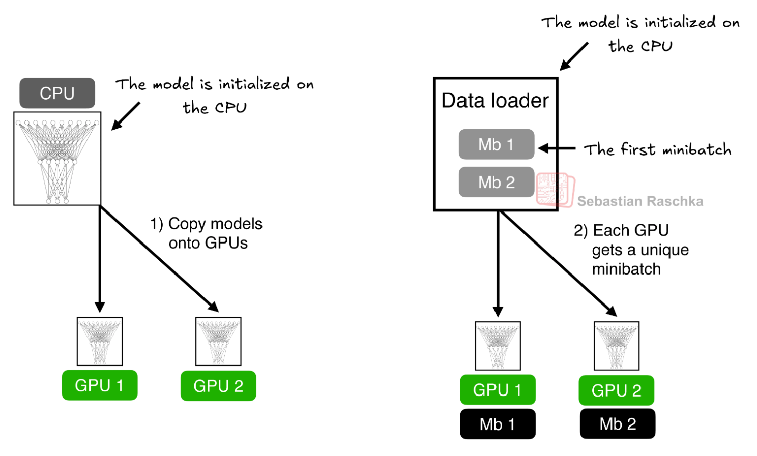Deep learning models involve massive matrix multiplications that run significantly faster on GPUs. GPUs have thousands of cores optimized for parallel computation.

9.1 CPU vs GPU Performance

Typical Speedups:

• Small models (< 1M parameters): 2-5× faster
• Medium models (1-50M parameters): 10-50× faster
• Large models (> 100M parameters): 50-100× faster

Why GPUs are Faster:

• Parallelism: CPUs have 4-16 cores; GPUs have 1000+ cores
• Memory Bandwidth: GPUs have 10-20× higher bandwidth (GB/s)
• Specialized Hardware: Tensor cores for matrix multiplication
• SIMD Operations: Single Instruction, Multiple Data

9.2 Moving to Device

To use a GPU, you must manually move both the neural network and the data tensors to the device.

Device Selection:

• "cuda": NVIDIA GPU (requires CUDA drivers)
• "mps": Apple Silicon (M1/M2/M3 Macs)
• "cpu": Fallback if no GPU available

Key Operations:

• model.to(device): Moves model parameters to device
• tensor.to(device): Moves data to device
• Move both model and data to the same device!

9.3 Memory Management on GPU

GPU Memory Breakdown:

• Model parameters (weights, biases)
• Activations (intermediate layer outputs for each batch)
• Gradients (same size as parameters)
• Optimizer state (Adam stores 2× parameters)

Example: ResNet-50 with batch size 32

• Parameters: 25.5M × 4 bytes = 102 MB
• Activations: ~200 MB (depends on input size)
• Gradients: 102 MB
• Optimizer (Adam): 204 MB
• Total: ~600 MB

Out of Memory? Try:

1. Reduce batch size (most effective)
2. Use gradient accumulation (simulate larger batches)
3. Use mixed precision training (float16)
4. Use gradient checkpointing (trade compute for memory)
5. Reduce model size

Monitoring GPU:

• NVIDIA: nvidia-smi command
• PyTorch: torch.cuda.memory_allocated(), torch.cuda.memory_reserved()

# Select device (reusing logic from Section 1)
if torch.cuda.is_available():
    device = torch.device("cuda")
    print(f"✓ Using NVIDIA GPU: {torch.cuda.get_device_name(0)}")
    print(f"  Total GPU Memory: {torch.cuda.get_device_properties(0).total_memory / (1024**3):.2f} GB")
elif torch.backends.mps.is_available():
    device = torch.device("mps")
    print("✓ Using Apple Silicon GPU (MPS)")
else:
    device = torch.device("cpu")
    print("⚠ No GPU available. Using CPU (training will be slower)")

print(f"  Device: {device}\n")

# 1. Move Model to Device
# This moves all model parameters (weights, biases) to the GPU
model.to(device)
print("✓ Model moved to device")

# Check model is on correct device
first_param_device = next(model.parameters()).device
print(f"  Model parameters are on: {first_param_device}\n")

# Calculate memory usage (approximate)
model_memory = sum(p.numel() * p.element_size() for p in model.parameters())
print(f"Model memory on device: {model_memory/1024:.2f} KB")

if device.type == "cuda":
    # Display GPU memory usage
    allocated = torch.cuda.memory_allocated(0) / (1024**2)  # MB
    reserved = torch.cuda.memory_reserved(0) / (1024**2)  # MB
    print(f"GPU Memory Allocated: {allocated:.2f} MB")
    print(f"GPU Memory Reserved: {reserved:.2f} MB\n")

# 2. Training Loop with Device Handling
print("="*60)
print("Training on device...")
print("="*60)

start_time = time.time()
model.train()  # Set to training mode

for epoch in range(2):  # Just 2 epochs for demonstration
    epoch_loss = 0.0
    
    for batch_idx, (inputs, targets) in enumerate(loader):
        # CRITICAL: Move Data to the same device as the model
        # Without this, you'll get "Expected all tensors to be on the same device" error
        inputs = inputs.to(device)
        targets = targets.to(device)

        # The rest of the loop is identical to CPU training
        outputs = model(inputs)
        loss = criterion(outputs, targets)
        optimizer.zero_grad()
        loss.backward()
        optimizer.step()
        
        epoch_loss += loss.item()
    
    avg_loss = epoch_loss / len(loader)
    print(f"Epoch {epoch+1}: Loss = {avg_loss:.4f}")

training_time = time.time() - start_time
print(f"\n✓ Training completed in {training_time:.2f}s")
print(f"  Device: {device}")

if device.type == "cuda":
    print(f"  Peak GPU Memory: {torch.cuda.max_memory_allocated(0) / (1024**2):.2f} MB")
    
    # Clear GPU cache
    torch.cuda.empty_cache()
    print("  GPU cache cleared")

# 3. Move model back to CPU for saving (optional, for compatibility)
print("\n" + "="*60)
print("Moving model back to CPU for saving...")
model_cpu = model.to('cpu')
torch.save(model_cpu.state_dict(), 'my_model.pth')
print("✓ Model saved (CPU version for compatibility)")

---

Conclusion

This tutorial covered the essential concepts of PyTorch for deep learning:

1. Tensors: The fundamental data structure for representing data and parameters
2. Automatic Differentiation: How PyTorch automatically computes gradients for backpropagation
3. Neural Networks: Building and understanding multilayer networks
4. Data Loading: Efficient batching and data handling
5. Training: The standard training loop with forward/backward passes
6. Model Persistence: Saving and loading trained models
7. FLOPS Analysis: Measuring and optimizing computational complexity
8. GPU Acceleration: Leveraging hardware for faster training

With these fundamentals, you’re ready to build, train, and deploy your own deep learning models using PyTorch!