(Adopted from https://github.com/ash80/RLHF_in_notebooks)

RLHF From Scratch: SFT → Reward Model → PPO, with GPT-2

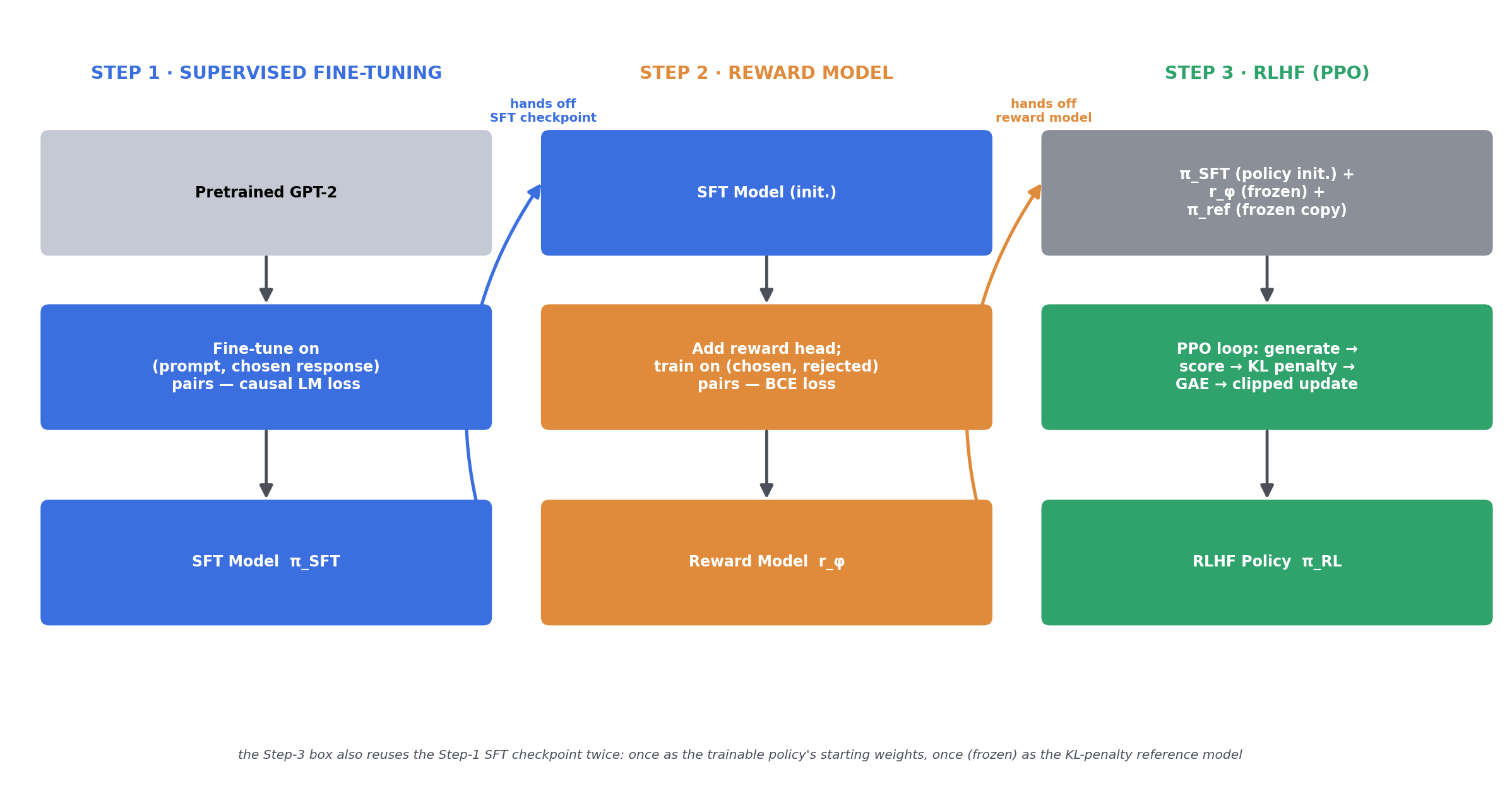
Reinforcement Learning from Human Feedback (RLHF) is the recipe that turns a raw, pretrained language model into something that follows instructions and produces outputs humans actually prefer. It’s a three-stage pipeline — supervised fine-tuning (SFT), reward model (RM) training, and reinforcement learning via PPO — and each stage feeds the next. This post walks through a from-scratch implementation of all three stages using GPT-2 (124M) and Hugging Face transformers, following the structure described in the InstructGPT / “N+ Implementation Details” paper. No trl library, no shortcuts — every loss function, every reward calculation, and every training loop is written out by hand so the mechanics are visible.

The three stages, in order:

1. SFT — teach a base language model to produce good responses by fine-tuning on (prompt, response) pairs.
2. Reward Model — train a separate model to score how good a response is, using human preference pairs (chosen vs. rejected).
3. RLHF (PPO) — use the reward model as a stand-in for human feedback and optimize the SFT model against it with proximal policy optimization, while a KL penalty keeps it from drifting too far from the SFT policy.

---

Stage 1: Supervised Fine-Tuning (SFT)

Base model and tokenizer

The starting point is gpt2, the smallest (124M parameter) checkpoint in the GPT-2 family. It’s decoder-only and autoregressive, which matters here: the same next-token-prediction objective used to pretrain it can be reused directly for fine-tuning, just on different data (prompt/response text instead of raw web text).

from transformers import AutoModelForCausalLM, AutoTokenizer
model_name = 'gpt2'
tokenizer = AutoTokenizer.from_pretrained(model_name)
model = AutoModelForCausalLM.from_pretrained(model_name)

GPT-2 uses byte-pair encoding (BPE), so text is split into subword pieces rather than whole words or characters, then mapped to integer token ids. Encoding and decoding round-trip losslessly.

Dataset

The dataset is Dahoas/synthetic-instruct-gptj-pairwise, a synthetic instruction-following preference dataset with ~33k examples. Each row has a short, single-turn prompt, a chosen (preferred) response, and a rejected (dispreferred) response — a reformatted relative of Anthropic’s HH-RLHF data. Since the dataset only ships a single train split, 10% is manually held out as validation:

from datasets import load_dataset
ds = load_dataset('Dahoas/synthetic-instruct-gptj-pairwise')
ds_split = ds['train'].train_test_split(test_size=0.1, seed=42)

ds_full_train = ds_split['train']   # prompt, chosen, rejected — reused later for RM training
ds_full_val   = ds_split['test']

# SFT only needs prompt + chosen response
ds_train = ds_full_train.remove_columns(['rejected']).rename_column('chosen', 'response')
ds_val   = ds_full_val.remove_columns(['rejected']).rename_column('chosen', 'response')

For SFT, only the chosen responses are used — the goal is to teach the model what a good answer looks like before reward modeling ever enters the picture. The seed=42 split is reused verbatim in the reward-model notebook, so the same held-out examples stay held out across the whole pipeline.

Formatting and tokenization

Each (prompt, response) pair is concatenated into a single string — prompt + <eos> + response — and tokenized as one sequence, rather than tokenizing prompt and response separately:

def tokenize(batch):
    texts = [prompt + tokenizer.eos_token + response
             for prompt, response in zip(batch['prompt'], batch['response'])]
    return tokenizer(texts)

tokenized_dataset_train = ds_train.map(
    tokenize, batched=True, batch_size=512,
    remove_columns=['prompt', 'response']
)

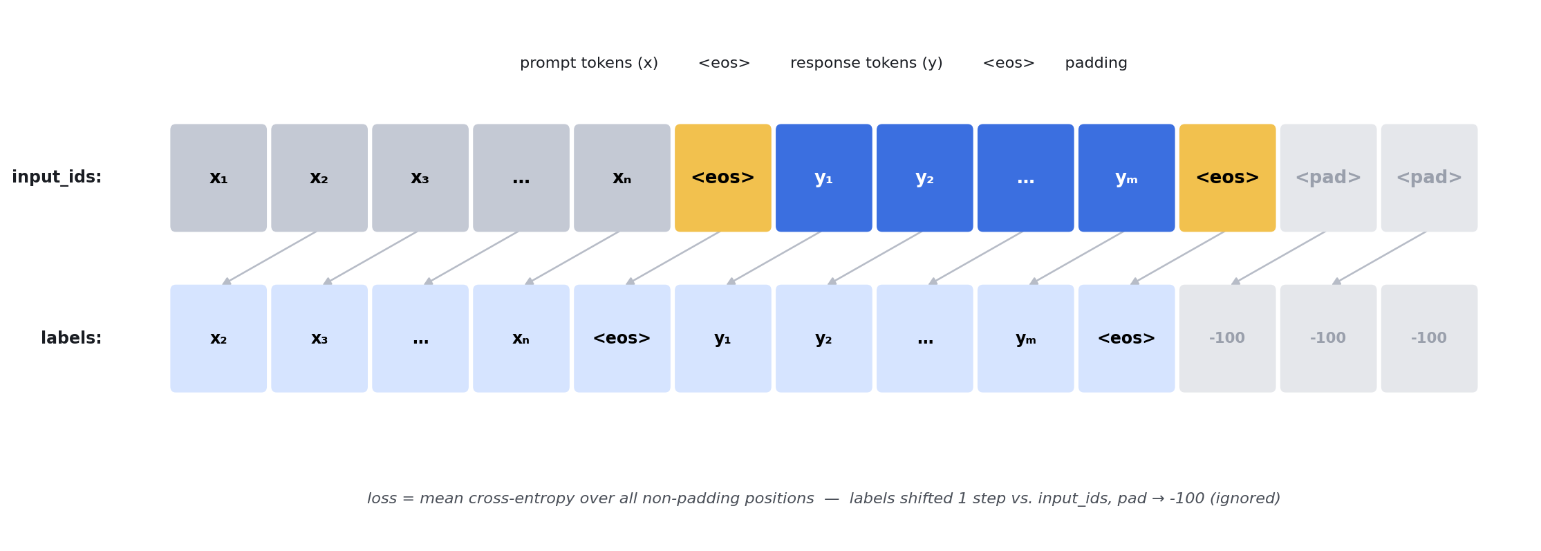
Training on this single concatenated sequence with a standard causal-LM loss teaches the model two things at once: to continue text like a prompt (leveraging pretraining), and — after seeing <eos> — to switch into “answering” mode and eventually emit <eos> again to stop.

Sequences are then filtered to between 9 and 128 tokens, trimming a small tail of unusually long examples while keeping most of the dataset.

The figure below shows the full token layout and how the loss mask lines up with it — labels[i] holds input_ids[i+1] (the next-token target), with -100 wherever that next token is itself padding:

Padding and the label mask

GPT-2 wasn’t pretrained with a dedicated pad token, so one has to be set explicitly before batches of variable-length sequences can be padded to a common width:

tokenizer.pad_token = tokenizer.eos_token

DataCollatorForLanguageModeling(tokenizer, mlm=False) then handles batch-level padding: it pads every example in a batch to the longest one, builds the matching attention_mask (1 for real tokens, 0 for padding), and produces a labels tensor — a copy of input_ids with padded positions replaced by -100, the value PyTorch’s cross-entropy loss is told to ignore. mlm=False selects causal (left-to-right) language modeling rather than BERT-style masked LM.

from torch.utils.data import DataLoader
from transformers import DataCollatorForLanguageModeling

data_collator = DataCollatorForLanguageModeling(tokenizer, mlm=False)
train_dataloader = DataLoader(tokenized_dataset_train, batch_size=32, collate_fn=data_collator)
val_dataloader = DataLoader(tokenized_dataset_val, batch_size=32, collate_fn=data_collator)

Training loop

Standard supervised fine-tuning: AdamW with lr=1e-4 — on the high end for full-model fine-tuning (typical full fine-tunes use 1e-5–5e-5), chosen here so a single epoch shows a visible change quickly, at the cost of noisier per-step loss.

import torch
optimizer = torch.optim.AdamW(model.parameters(), lr=1e-4)
num_epochs = 1

device = torch.device('mps' if torch.backends.mps.is_available() else 'cuda' if torch.cuda.is_available() else 'cpu')
model.to(device)

validate(0)  # untrained baseline
for epoch in range(num_epochs):
    model.train()
    for batch in train_dataloader:
        batch = batch.to(device)
        outputs = model(**batch)          # internally shifts input_ids vs. labels for next-token loss
        loss = outputs.loss
        optimizer.zero_grad()
        loss.backward()
        optimizer.step()
    validate(epoch + 1)

model(**batch) internally shifts input_ids by one position against labels to compute the next-token loss (ForCausalLMLoss in transformers). Validation runs in model.eval() / torch.no_grad() mode — no dropout, no autograd graph — and is called once before training (epoch-0 baseline) and once after each epoch.

The training objective is the standard autoregressive (causal) language-modeling loss — negative log-likelihood of each response token given the prompt and all preceding tokens:

where $x$ is the prompt, $y = (y_1, \dots, y_T)$ is the tokenized response, and $\pi_\theta$ is the model’s next-token probability distribution. In practice this is computed as the mean cross-entropy over all non-padding token positions in a batch, with padding positions excluded via the labels = -100 mask.

Results and a known failure mode

Validation loss dropped from 3.96 → 2.19 after one epoch on a filtered ~26.5k-example slice. Qualitatively, the model stayed on-topic (e.g. correctly discussing yoga for arthritis, or the atomic mass of lithium) — confirming the loss drop reflects real instruction-following. But with greedy decoding (do_sample=False), every response eventually degenerated into a repetition loop (e.g. repeating “This is equal to 0.5235 grams.” verbatim).

This is expected, not a broken run, for two compounding reasons:

Greedy decoding is repetition-prone by construction — once a phrase repeats, it becomes the highest-probability next token again, so the model gets stuck. Fixes: no_repeat_ngram_size=3, repetition_penalty=1.3, or switch to sampling (do_sample=True, top_p=0.9, temperature=0.8). Second, one epoch on a length-filtered dataset at a relatively high learning rate teaches the style of a short response but not reliably when to stop — more epochs or a less aggressive length filter would tighten this up.

The checkpoint is saved in standard Hugging Face format for reuse in the next two stages:

model.save_pretrained('./sft_model_epoch_1')

---

Stage 2: Reward Model Training

Why a reward model

PPO (Stage 3) needs a scalar reward signal for arbitrary generated text, but human labels are expensive to collect at RL scale. The standard RLHF solution is to train a model that predicts human preference — a stand-in for a human rater that can be queried as often as needed during policy optimization.

Building preference pairs

Training a reward model requires preference pairs, not text-to-text examples: two responses to the same prompt, one preferred over the other. The same dataset and same seed=42 split from SFT is reused, and make_preference_pairs turns each example into two rows — the chosen response with label=1 and the rejected response with label=0:

def make_preference_pairs(ds):
    n = len(ds)
    prompts, chosen, rejected = ds['prompt'], ds['chosen'], ds['rejected']
    return Dataset.from_dict({
        'prompt': prompts + prompts,
        'response': chosen + rejected,
        'label': [1] * n + [0] * n,
    })

ds_train = make_preference_pairs(ds_split['train'].select(range(10000)))
ds_val   = make_preference_pairs(ds_split['test'].select(range(1000)))

This doubles the dataset size (10k → 20k rows) and gives the model a genuine notion of reward: score the response people actually preferred higher than the one they didn’t, for the same prompt — both responses are real human-ranked answers from the original HH-RLHF collection, not a mismatched pairing.

Tokenization with a reward token

Same prompt + <eos> + response framing as SFT, plus one addition: a REWARD_TOKEN_ID (set equal to eos_token_id) is appended to the very end of every sequence, and score_index records its position:

REWARD_TOKEN_ID = tokenizer.eos_token_id

def tokenize(batch):
    texts = [prompt + tokenizer.eos_token + response
             for prompt, response in zip(batch['prompt'], batch['response'])]
    outputs = tokenizer(texts)
    outputs['score'] = [0] * len(outputs['input_ids'])
    outputs['score_index'] = [0] * len(outputs['input_ids'])
    for i in range(len(outputs['input_ids'])):
        outputs['input_ids'][i].append(REWARD_TOKEN_ID)
        outputs['attention_mask'][i].append(1)
        outputs['score'][i] = float(batch['label'][i])
        outputs['score_index'][i] = len(outputs['input_ids'][i]) - 1
    return outputs

That final position’s hidden state — computed only after the model has attended over the entire prompt and response — is what the reward head reads from. This conditions the reward score on the whole (prompt, response) pair rather than any single mid-sequence token.

Architecture: GPT-2 + reward head

The reward model wraps GPT-2 with a linear head that maps each position’s hidden state to a scalar, then applies a sigmoid to squash it into [0, 1]:

class RewardHead(nn.Module):
    def __init__(self, config):
        super().__init__()
        self.hidden_size = config.hidden_size
        self.reward = nn.Linear(self.hidden_size, 1)
        nn.init.normal_(self.reward.weight, std=(1.0 / np.sqrt(self.hidden_size + 1)))
        nn.init.zeros_(self.reward.bias)

    def forward(self, hidden_states):
        return self.reward(hidden_states)

class GPT2RewardHead(nn.Module):
    def __init__(self, model_name):
        super().__init__()
        self.llm = AutoModelForCausalLM.from_pretrained(model_name)
        self.reward_head = RewardHead(self.llm.config)

    def forward(self, input_ids, attention_mask):
        transformer_outputs = self.llm.forward(
            input_ids=input_ids, attention_mask=attention_mask, output_hidden_states=True
        )
        last_hidden_state = transformer_outputs.hidden_states[-1]
        reward = self.reward_head(last_hidden_state).squeeze(-1)
        return torch.sigmoid(reward)

Formally, the reward model $r_\phi$ is a linear projection of the final hidden state $h_T$ at the reward-token position, squashed through a sigmoid:

so $r_\phi(x,y) \in (0, 1)$.

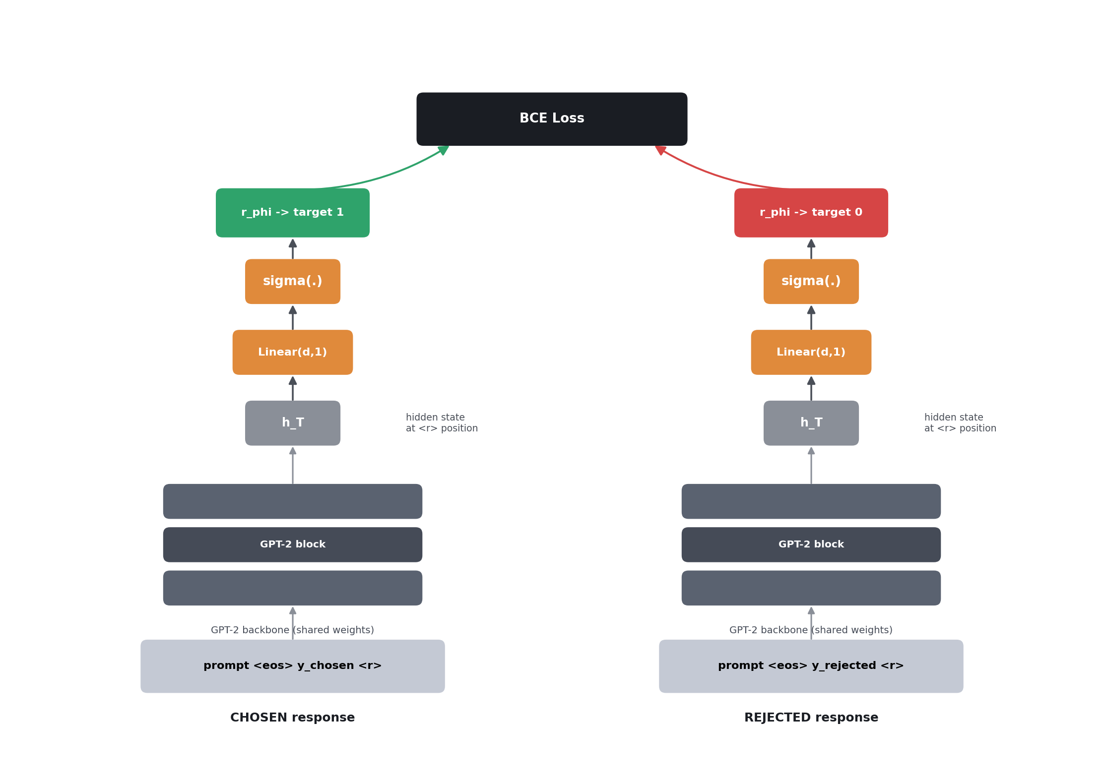
The model is initialized from rinabuoy/gpt2-sft — the SFT checkpoint from Stage 1 — rather than the raw pretrained checkpoint, so the reward model starts from a model that already understands the instruction-response format it’s scoring.

Loss: binary classification (BCE)

Since each row is labeled 1 (chosen) or 0 (rejected), training reduces to binary classification with BCE loss, applied only at the score_index position of each sequence:

optimizer = torch.optim.AdamW(model.parameters(), lr=1e-4)
criterion = nn.BCELoss()
num_epochs = 1

for epoch in range(num_epochs):
    model.train()
    for batch in train_dataloader:
        inputs = batch.to(device)
        scores = model(inputs['input_ids'], inputs['attention_mask'])
        batch_indices = torch.arange(scores.shape[0])
        score = scores[batch_indices, inputs['score_index']]
        target = inputs['score']
        loss = criterion(score, target)
        optimizer.zero_grad()
        loss.backward()
        optimizer.step()

The BCE loss for a single labeled example $(x, y, l)$, with $l \in \{0, 1\}$, is:

Note this differs from the pairwise ranking loss used in the original InstructGPT paper, which compares a chosen/rejected pair directly within a single training example:

Here chosen/rejected are instead treated as independent binary-labeled examples rather than compared directly within a pair, which is simpler to implement but only implicitly encourages chosen to score higher than rejected for the same prompt.

Evaluation

Two checks confirm the reward model learned something sensible. A confusion matrix on held-out preference labels (thresholding the sigmoid score at 0.5) gives a coarse accuracy signal. More intuitively, scoring the chosen and rejected response to the same held-out prompt side by side should consistently rank chosen higher:

def reward_for(prompt, response):
    enc = tokenizer(prompt + tokenizer.eos_token + response, return_tensors='pt')
    input_ids = torch.cat([enc['input_ids'], torch.tensor([[REWARD_TOKEN_ID]])], dim=1)
    attention_mask = torch.cat([enc['attention_mask'], torch.tensor([[1]])], dim=1)
    scores = model(input_ids.to(device), attention_mask.to(device))
    return scores[0, -1].item()

The checkpoint is saved as a raw state dict (torch.save(model.state_dict(), 'reward_model.pt')), since GPT2RewardHead is a custom nn.Module, not a Hugging Face PreTrainedModel — reloading it means reconstructing the wrapper class first, then loading weights into it.

---

Stage 3: RLHF with PPO

This is where the SFT model and reward model come together. The SFT checkpoint becomes the policy being optimized, the reward model scores its outputs, and Proximal Policy Optimization (PPO) provides the update rule — with a KL penalty against the original SFT model to prevent the policy from over-optimizing against the reward model’s blind spots.

Framing RLHF as an MDP

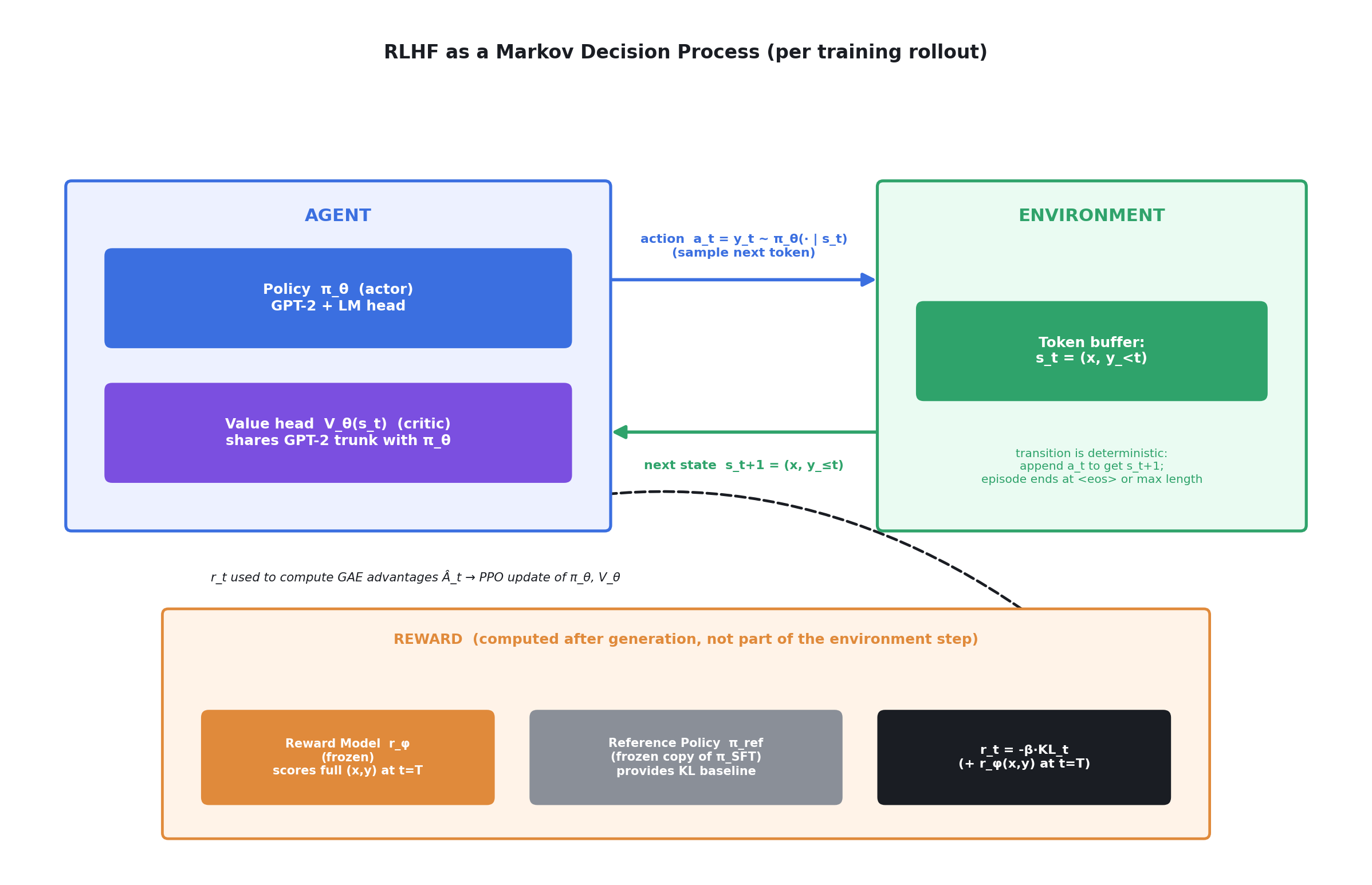
Before looking at code, it’s worth being precise about what the reinforcement-learning problem actually is here, since “prompt in, text out” doesn’t immediately look like an RL environment. Casting text generation as a Markov Decision Process (MDP):

• State $s_t$ — the prompt plus every token generated so far, $s_t = (x, y_{<t})$. State $s_0$ is just the prompt $x$.
• Action $a_t$ — the next token, $a_t = y_t$, sampled from the policy’s distribution over the vocabulary, $\pi_\theta(\cdot \mid s_t)$.
• Transition — deterministic: the environment appends $a_t$ to $s_t$ to get $s_{t+1}$. There’s no external world dynamics to learn, unlike robotics or games — the only thing being learned is which token to pick.
• Episode termination — the episode ends when the policy emits <eos> or a maximum length is reached.
• Reward $r_t$ — zero at every intermediate step except a per-token KL penalty against the frozen reference policy; the reward model’s score is added once, at the final step $T$, since that’s the only point at which a full response exists to score.
• Policy (actor) $\pi_\theta$ — the GPT-2 language model being trained; its LM head defines the action distribution.
• Value function (critic) $V_\theta(s_t)$ — the value head, sharing GPT-2’s trunk with the policy, estimating expected future reward from state $s_t$. Used to compute advantages, not to select actions.

The reward model and the reference policy are both frozen — they define the reward function but are never updated by gradient descent themselves; only $\pi_\theta$ (and its attached value head) are trained.

Two model wrappers

The reward model is reloaded exactly as trained in Stage 2 (GPT2RewardModel, sigmoid output in [0, 1]) and kept frozen throughout — it is only ever used to score generations, never updated.

The policy is the SFT checkpoint wrapped with a value head instead of a reward head — this is what PPO actually trains:

class ValueHead(nn.Module):
    def __init__(self, config):
        super().__init__()
        self.value = nn.Linear(config.hidden_size, 1)
        nn.init.normal_(self.value.weight, std=(1.0 / np.sqrt(config.hidden_size + 1)))
        nn.init.zeros_(self.value.bias)

    def forward(self, hidden_states):
        return self.value(hidden_states)

class ModelForCausalLMWithValueHead(nn.Module):
    def __init__(self, model_path):
        super().__init__()
        self.llm = AutoModelForCausalLM.from_pretrained(model_path)
        self.v_head = ValueHead(self.llm.config)

    def forward(self, input_ids, attention_mask):
        out = self.llm.forward(input_ids, attention_mask=attention_mask, output_hidden_states=True)
        lm_logits = out.logits
        value = self.v_head(out.hidden_states[-1]).squeeze(-1)
        return lm_logits, value

    def generate(self, *args, **kwargs):
        return self.llm.generate(*args, **kwargs)

model = ModelForCausalLMWithValueHead('rinabuoy/gpt2-sft')

The value head estimates the expected future reward from any point in a generated sequence — it’s the “critic” half of PPO’s actor-critic setup, trained jointly with the language-modeling logits (the “actor”).

A frozen deep copy of the policy, sft_model = deepcopy(model), is kept as the reference model purely for computing the KL penalty below; its weights never update.

Dataset and query construction

The same Dahoas/synthetic-instruct-gptj-pairwise split is reused, filtered to prompts longer than 8 words, then truncated to a short random-length prefix (2–7 tokens) to form the RL “query” — the model has to generate a continuation, not just reproduce a fixed prompt:

input_token_length_range = list(range(2, 8))

def tokenize(sample):
    input_size = random.choice(input_token_length_range)
    sample['input_ids'] = tokenizer.encode(sample['prompt'])[:input_size]
    sample['attention_mask'] = [1] * len(sample['input_ids'])
    sample['query'] = tokenizer.decode(sample['input_ids'])
    return sample

Generation length is also randomized per example (5–15 new tokens) using sampling (do_sample=True, top_k=0, top_p=1.0 — i.e. unrestricted sampling from the full softmax), which produces the exploration PPO needs.

Computing the reward: reward-model score minus KL penalty

This is the core RLHF equation. For a full (prompt, response) pair $(x, y)$, the total episode reward combines the reward model’s score with a KL penalty against the reference (SFT) policy:

Since an exact sequence-level KL is intractable, it’s approximated per-token along the sampled trajectory and distributed across timesteps as an intermediate reward:

with $\beta = 0.2$. That is, every generated token pays a small per-token KL cost, and the reward model’s scalar score is added only at the final token $T$ of the response — matching rewards[j, end - 1] += score_tensors[j] in the code below. The reward model’s score alone isn’t used directly as the RL reward. Instead, a per-token KL divergence between the current policy’s and the frozen reference model’s output distributions is subtracted at every generated token, and the reward model’s score is added only at the final token of the response:

def compute_rewards(input_data, query_tensors, response_tensors, score_tensors):
    with torch.no_grad():
        logits, values = model(**input_data)
        ref_logits, _ = sft_model(**input_data)

        logp = F.log_softmax(logits[:, :-1, :], dim=-1)
        ref_logp = F.log_softmax(ref_logits[:, :-1, :], dim=-1)
        labels = input_data['input_ids'][:, 1:]

        logp = torch.gather(logp, 2, labels.unsqueeze(-1)).squeeze(-1)
        ref_logp = torch.gather(ref_logp, 2, labels.unsqueeze(-1)).squeeze(-1)

        kl = logp - ref_logp
        beta = 0.2
        rewards = -beta * kl                       # per-token KL penalty

        masks = attention_mask[:, 1:].clone()
        for j in range(len(query_tensors)):
            start = len(query_tensors[j]) - 1
            end = start + len(response_tensors[j])
            masks[j, :start] = 0                    # mask out the query/prompt tokens
            masks[j, end:] = 0                       # mask out padding after the response
            rewards[j, end - 1] += score_tensors[j]  # reward-model score lands on the last response token
            rewards[j, :] *= masks[j, :]

    return logp, rewards, values[:, :-1], masks

The reward-model’s raw sigmoid score is rescaled from [0, 1] to [-1, 1] before this (score = 2 * (score - 0.5)), and β = 0.2 controls how strongly the policy is penalized for diverging from the SFT reference — too high and the model can’t improve past SFT; too low and it can “reward hack” the RM by drifting into degenerate text the RM happens to score well but which no longer resembles coherent language.

Concretely, for a short rollout from the prompt "This movie was", the states, actions, and rewards line up like this:

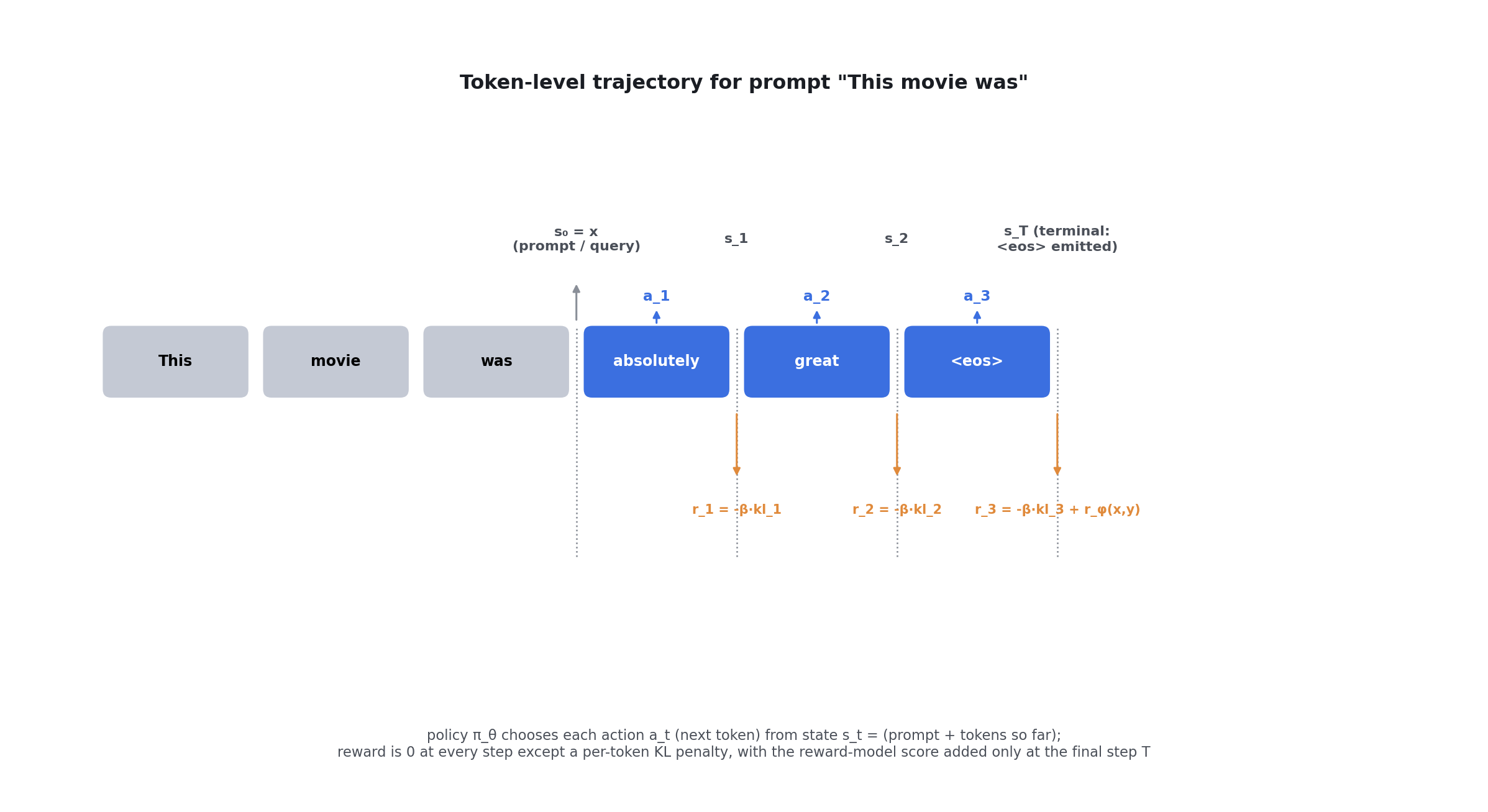
Every generated token is one action; the state right after it is what the policy conditions on for the next action; and only the very last transition receives the reward model’s actual judgment of the completed response.

Advantage estimation: GAE

Per-token rewards and value estimates are converted into advantages using Generalized Advantage Estimation (GAE), with γ = 1.0 (no discounting) and λ = 0.95:

def compute_advantage(rewards, values, masks):
    lastgae = 0.0
    advantage_reversed = []
    gamma, lam = 1.0, 0.95
    for t in reversed(range(rewards.shape[-1])):
        nextvalues = values[:, t + 1] if t < rewards.shape[-1] - 1 else 0.0
        delta = rewards[:, t] + gamma * nextvalues - values[:, t]
        lastgae = delta + gamma * lam * lastgae
        advantage_reversed.append(lastgae)
    advantages = torch.stack(advantage_reversed[::-1], dim=1)
    advantages = masked_whiten(advantages, masks)   # normalize to zero mean, unit variance over real (non-masked) tokens
    returns = advantages + values
    return advantages, returns

Formally, GAE computes the temporal-difference residual at each step,

and the advantage as an exponentially-weighted sum of future residuals, computed efficiently via the backward recursion:

with $\gamma = 1.0$ and $\lambda = 0.95$ here. The value-function regression target (“return”) is then the advantage plus the baseline value estimate:

Advantages are whitened (mean-centered, variance-normalized) over the masked (non-padding) tokens only, which stabilizes the policy gradient magnitude across batches:

where $\mu_{\hat A}$ and $\sigma^2_{\hat A}$ are the mean and variance of $\hat A$ taken only over unmasked (real, non-padding) token positions.

The PPO update

The clipped surrogate objective compares the new policy’s log-probabilities against the log-probabilities recorded before any updates this round (old_logprobs), preventing any single update from moving the policy too far:

cliprange_ratio = 0.2
v_loss_coeff = 0.1
ratio_threshold = 10

def compute_loss(old_logprobs, values, logprobs, vpreds, masks, advantages, returns):
    ratio = torch.exp(logprobs - old_logprobs)
    pg_loss1 = -ratio * advantages
    pg_loss2 = -torch.clamp(ratio, 1 - cliprange_ratio, 1 + cliprange_ratio) * advantages
    pg_loss = masked_mean(torch.max(pg_loss1, pg_loss2), masks)

    v_loss = masked_mean((vpreds - returns) ** 2, masks)
    loss = pg_loss + v_loss_coeff * v_loss

    # safety valve: skip the update entirely if the policy has moved implausibly far
    if masked_mean(ratio, masks) > ratio_threshold:
        return loss * 0.0, v_loss * 0.0
    return loss, v_loss

Formally, with the importance-sampling ratio between the updated and old policy,

the clipped surrogate policy objective is

with clip range $\epsilon = 0.2$ (cliprange_ratio). The value-function loss is a simple squared-error regression toward the GAE return:

and the total loss minimized each PPO mini-batch step combines both (note the sign flip, since $L^{\text{CLIP}}$ is framed as an objective to maximize):

This is the standard PPO-clip objective (pg_loss) plus an MSE value-function loss (v_loss, weighted by v_loss_coeff = 0.1), combined into a single scalar. The ratio_threshold guard zeroes out the entire update if the importance-sampling ratio blows up — a defensive measure against destabilizing gradient spikes.

Each PPO round runs several epochs over the same batch of generated rollouts, in shuffled mini-batches — reusing the same rollouts multiple times is what makes PPO more sample-efficient than vanilla policy gradient:

mini_batch_size = 4
ppo_epochs = 4

def mini_batch_train():
    for ep in range(ppo_epochs):
        batch_inds = np.random.permutation(batch_size)
        for start in range(0, batch_size, mini_batch_size):
            mb_inds = batch_inds[start:start + mini_batch_size]
            mb_logits, mb_vpreds = model(input_data['input_ids'][mb_inds], input_data['attention_mask'][mb_inds])
            mb_logprobs = torch.gather(
                F.log_softmax(mb_logits[:, :-1, :], dim=-1), 2,
                input_data['input_ids'][mb_inds][:, 1:].unsqueeze(-1)
            ).squeeze(-1)
            loss, v_loss = compute_loss(
                logprobs[mb_inds], values[mb_inds], mb_logprobs, mb_vpreds[:, :-1],
                masks[mb_inds], advantages[mb_inds], returns[mb_inds]
            )
            optimizer.zero_grad()
            loss.backward()
            optimizer.step()

The full RLHF loop

Putting it together, one epoch over the training data does, per batch: generate responses from the current policy, score them with the frozen reward model, compute per-token KL-adjusted rewards against the frozen reference model, compute GAE advantages, then run several PPO mini-batch epochs on that batch of rollouts before moving to the next batch:

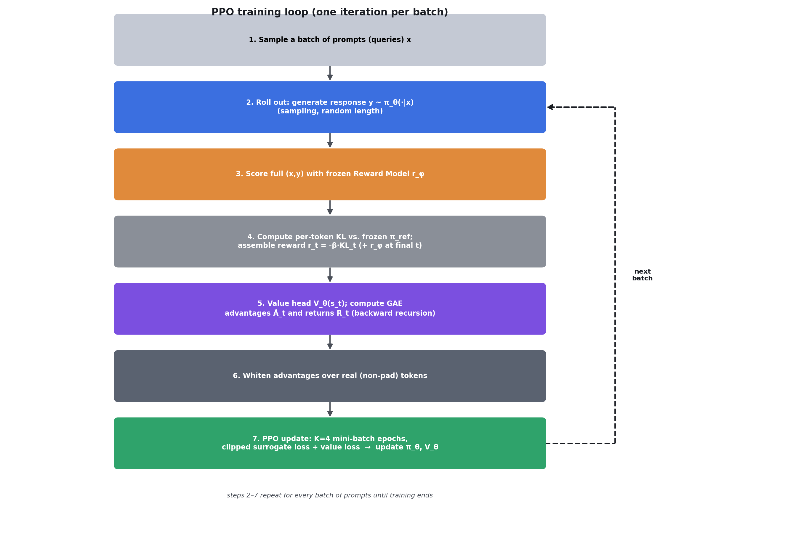
learning_rate = 1e-5
optimizer = torch.optim.AdamW(model.parameters(), lr=learning_rate)

for epoch in range(num_epochs):
    for batch in train_dataloader:
        # 1. Generate responses from the current policy
        response_tensors, query_response_tensors, score_tensors = [], [], []
        for i, query in enumerate(batch['input_ids']):
            query_response = model.generate(input_ids=query.unsqueeze(0), ..., **generation_kwargs).squeeze(0)
            query_response_tensors.append(query_response)
            # 2. Score with the frozen reward model
            score = reward_model(torch.cat([query_response, eos]).unsqueeze(0), ...).squeeze(0)[-1]
            score_tensors.append(2 * (score - 0.5))

        input_data = data_collator([...])  # pad the batch of query+response sequences

        # 3. KL-adjusted rewards and GAE advantages
        logprobs, rewards, values, masks = compute_rewards(input_data, query_tensors, response_tensors, score_tensors)
        advantages, returns = compute_advantage(rewards, values, masks)

        # 4. PPO mini-batch updates
        mini_batch_train()

Note the much lower learning rate here (1e-5) than SFT or RM training (1e-4) — PPO updates are inherently noisier (they depend on sampled rollouts and an estimated advantage, not a fixed supervised target), so a smaller step size is needed for stability.

Validation

Since there’s no held-out “correct answer” for RL, validation instead generates responses to held-out prompts and reports the average reward-model score — a rising average score is the signal that PPO is doing its job:

def validate():
    scores = []
    for batch in val_dataloader:
        for query in batch['input_ids']:
            query_response = model.generate(...)
            score = reward_model(...)
            scores.append((2 * (score - 0.5)).item())
    print('avg score:', sum(scores) / len(scores))

The PPO-trained policy (ppo_model_epoch_1.pt) can then be compared directly against the pre-PPO SFT checkpoint by running validate() against both — the expected outcome is a higher average reward-model score after PPO, reflecting outputs the reward model (and by extension, the human preferences it was trained on) rates more highly.

Inference

At inference time, prompts are short sentence-fragment continuations rather than full instructions (matching how the PPO stage was trained on this dataset’s prompts), and each generated completion can be scored on the spot with the reward model to sanity-check the RLHF stage actually improved things:

def score_response(prompt, response):
    query_response = tokenizer(prompt + response, return_tensors='pt')['input_ids'][0]
    query_response_score = torch.cat([query_response, torch.tensor([REWARD_TOKEN_ID])])
    score = reward_model(query_response_score.unsqueeze(0), torch.ones_like(query_response_score).unsqueeze(0))
    return (2 * (score[0, -1] - 0.5)).item()

# 'This movie was' -> completion, reward score

---

Putting the pipeline together

The three stages form a strict dependency chain: SFT teaches the base model the target response format and style; the reward model learns to score responses in that same format, using human preference labels as ground truth; and PPO then optimizes the SFT policy against the reward model’s scores, with a KL penalty tethering it back to the SFT model so it can’t “hack” the reward model by drifting into text the RM was never trained to judge well.

A few implementation choices are worth calling out because they diverge from naive intuition:

The reward model here uses independent BCE loss on chosen/rejected rows rather than a pairwise ranking loss — simpler to implement, and it still works in practice because both rows for the same prompt appear in training, but it doesn’t explicitly enforce the ranking the way -log σ(r_chosen - r_rejected) does.

The KL penalty is computed per-token throughout the whole sequence, but the reward-model score is injected only once, at the final response token — the reward model saw the whole response before assigning that score, so it makes sense for the reward signal to land only once the full response has actually been produced.

Learning rates differ meaningfully across stages: 1e-4 for both SFT and RM training (fast convergence on straightforward supervised objectives), but 1e-5 for PPO, reflecting the higher variance of policy-gradient updates on sampled rollouts.

This whole pipeline is a minimal, from-scratch RLHF implementation — no trl, no accelerate, and a 124M-parameter model — so it trains and iterates fast, but it’s making the same tradeoffs at a much smaller scale as production RLHF systems: a KL-regularized policy-gradient objective (PPO), a learned reward model in place of a human rater, and a value function trained jointly to reduce gradient variance.