Understanding Transformers in Deep Learning
Published on Thursday, 26-06-2025
(Adopted from CS224N and MIT6S191)
Transformers have revolutionized deep learning, particularly in natural language processing (NLP) and computer vision. This blog post explores the key concepts from a lecture on transformers, covering feedforward layers, recurrent neural networks (RNNs), attention mechanisms, and the transformer architecture itself. We’ll also dive into advanced variants like Vision Transformers (ViT), Pre-Norm Transformers, RMSNorm, SwiGLU MLP, and Mixture of Experts (MoE). For each concept, I’ll provide detailed explanations and, where applicable, PyTorch code to illustrate their implementation.
1. Feedforward Neural Networks
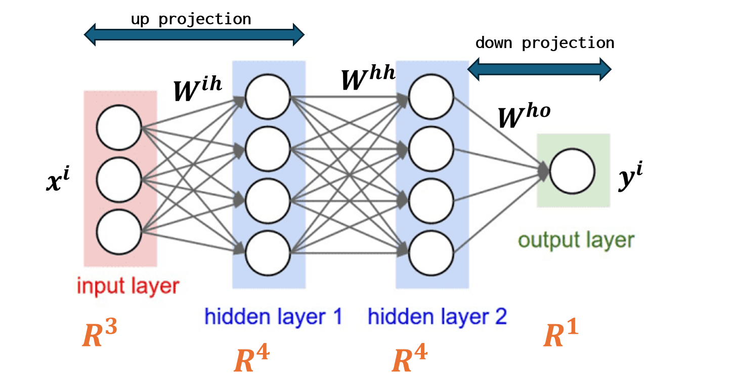
Feedforward neural networks (FFNNs) are the foundation of many deep learning models. They consist of layers where information flows in one direction, from input to output, through a series of transformations.
- Up Projection: The input vector is transformed into a higher-dimensional space using a weight matrix.
- Hidden Layers: Multiple hidden layers process the data, often with non-linear activation functions like ReLU.
- Down Projection: The output is mapped back to the desired dimension.
Here’s a simple PyTorch implementation of a feedforward layer:
import torch
import torch.nn as nn

class FeedForward(nn.Module):
    def __init__(self, input_dim, hidden_dim, output_dim):
        super(FeedForward, self).__init__()
        self.up_projection = nn.Linear(input_dim, hidden_dim)
        self.relu = nn.ReLU()
        self.down_projection = nn.Linear(hidden_dim, output_dim)

    def forward(self, x):
        x = self.up_projection(x)
        x = self.relu(x)
        x = self.down_projection(x)
        return x

# Example usage
model = FeedForward(input_dim=128, hidden_dim=512, output_dim=128)
x = torch.randn(32, 128)  # Batch of 32 vectors of size 128
output = model(x)
print(output.shape)  # torch.Size([32, 128])
This code defines a feedforward network with an up projection to a hidden dimension, a ReLU activation, and a down projection back to the output dimension.
2. Recurrent Neural Networks (RNNs)
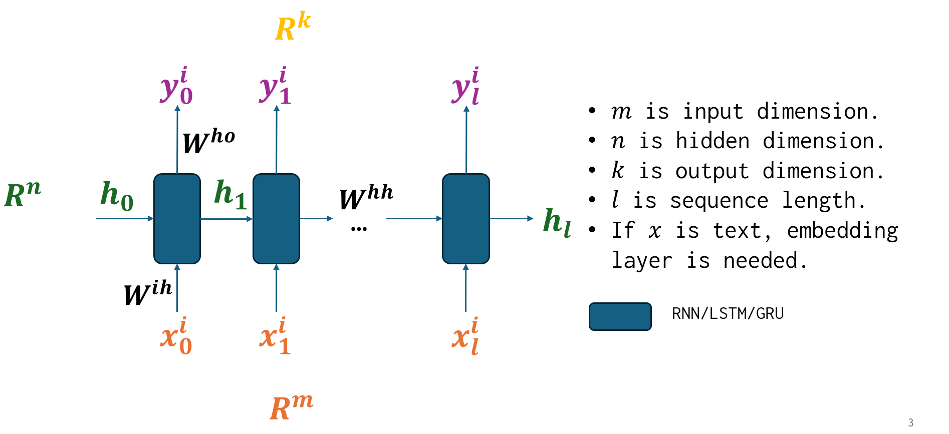
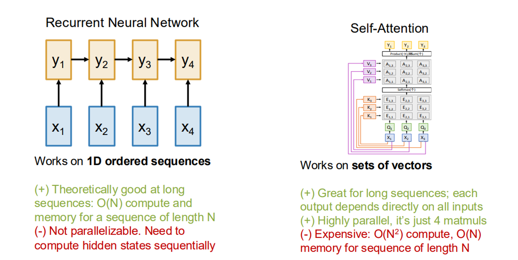
RNNs are designed for sequential data, such as time series or text, where the output of one step is fed as input to the next. They maintain a hidden state that captures information from previous time steps, making them theoretically suitable for long sequences. However, they suffer from issues like vanishing gradients and sequential computation, which limits parallelization.
- Advantages: compute and memory for a sequence of length , good for capturing sequential dependencies.
- Disadvantages: Not parallelizable due to sequential processing of hidden states.
Here’s a basic RNN implementation in PyTorch:
class SimpleRNN(nn.Module):
    def __init__(self, input_size, hidden_size, output_size):
        super(SimpleRNN, self).__init__()
        self.rnn = nn.RNN(input_size, hidden_size, batch_first=True)
        self.fc = nn.Linear(hidden_size, output_size)

    def forward(self, x):
        h0 = torch.zeros(1, x.size(0), self.rnn.hidden_size)  # Initial hidden state
        out, _ = self.rnn(x, h0)  # RNN output
        out = self.fc(out[:, -1, :])  # Take the last time step
        return out

# Example usage
rnn = SimpleRNN(input_size=10, hidden_size=20, output_size=5)
x = torch.randn(32, 50, 10)  # Batch of 32 sequences, each of length 50
output = rnn(x)
print(output.shape)  # torch.Size([32, 5])
This RNN processes sequences with a hidden state, but its sequential nature makes it less efficient for long sequences compared to transformers.
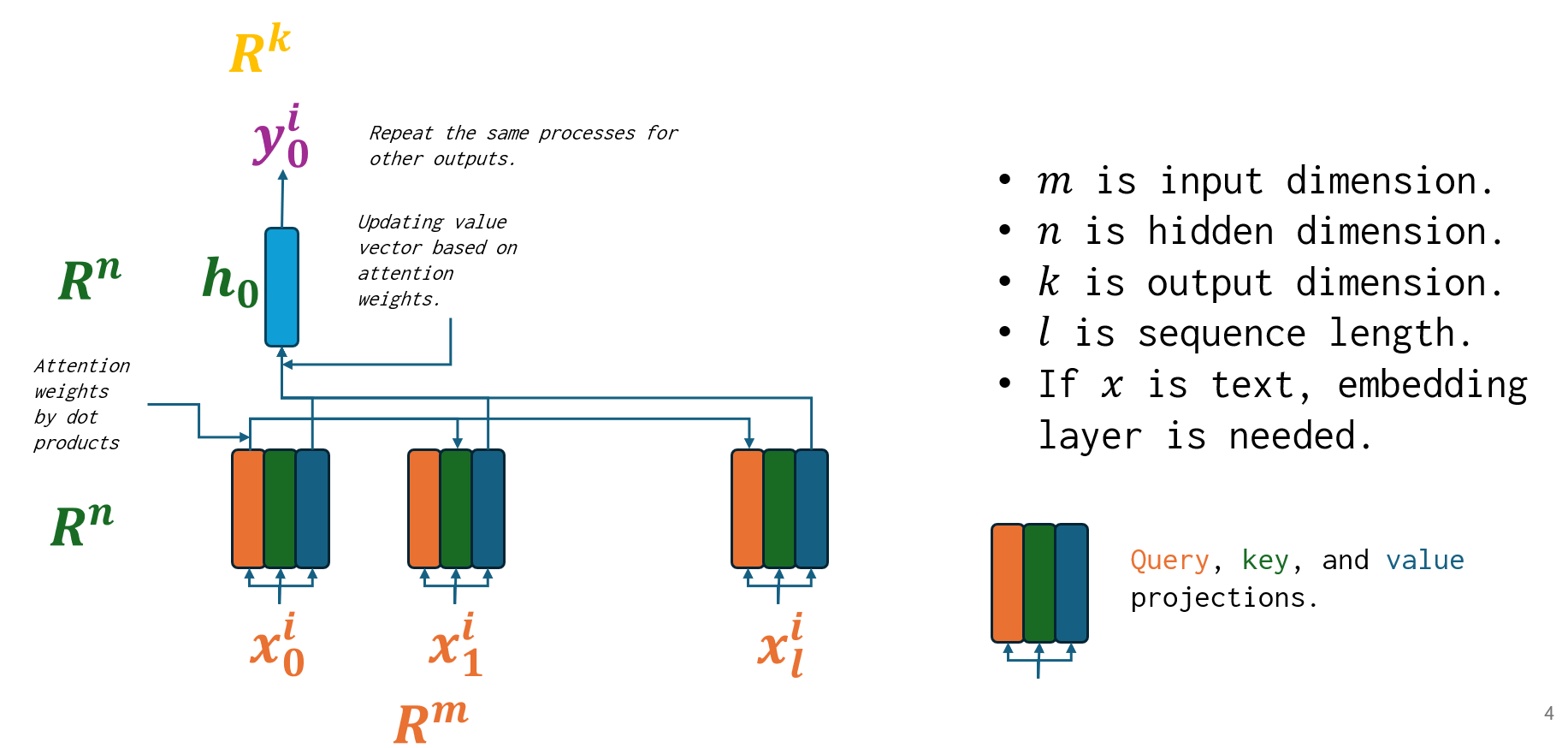
3. Attention Mechanisms
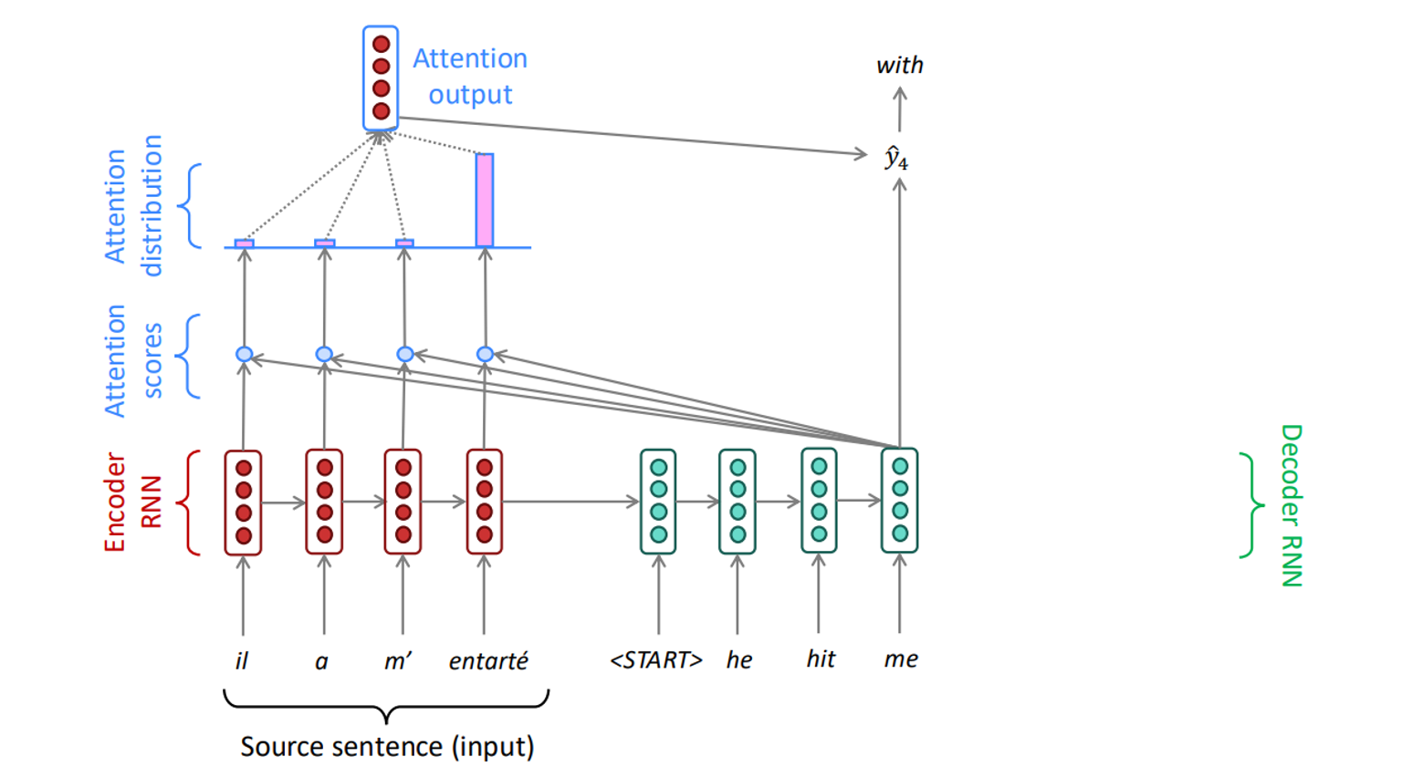
Attention mechanisms allow models to focus on specific parts of the input when making predictions, rather than relying solely on the entire sequence. They are particularly useful in sequence-to-sequence tasks like translation.
The attention process involves:
- Computing attention scores , where is the decoder’s hidden state at time , and are encoder hidden states.
- Applying softmax to get attention weights: .
- Using these weights to compute a weighted sum of encoder hidden states: .
- Concatenating with to proceed with decoding: .
Here’s a PyTorch implementation of a basic attention mechanism:
class Attention(nn.Module):
    def __init__(self, hidden_size):
        super(Attention, self).__init__()
        self.hidden_size = hidden_size

    def forward(self, decoder_hidden, encoder_outputs):
        # decoder_hidden: [batch_size, hidden_size]
        # encoder_outputs: [batch_size, seq_len, hidden_size]
        energies = torch.bmm(decoder_hidden.unsqueeze(1), encoder_outputs.transpose(1, 2))  # [batch_size, 1, seq_len]
        attention_weights = torch.softmax(energies, dim=-1)  # [batch_size, 1, seq_len]
        context = torch.bmm(attention_weights, encoder_outputs)  # [batch_size, 1, hidden_size]
        return context.squeeze(1), attention_weights.squeeze(1)

# Example usage
attention = Attention(hidden_size=128)
decoder_hidden = torch.randn(32, 128)
encoder_outputs = torch.randn(32, 50, 128)
context, weights = attention(decoder_hidden, encoder_outputs)
print(context.shape, weights.shape)  # torch.Size([32, 128]), torch.Size([32, 50])
This attention mechanism computes scores between the decoder’s hidden state and encoder outputs, producing a context vector and attention weights.
RNN vs. Attention
RNNs
- Pros: Efficient for long sequences ($ O(N) $ compute and memory), theoretically good at capturing sequential dependencies.
- Cons: Not parallelizable due to sequential hidden state updates.
Self-Attention
- Pros: Highly parallelizable, each output depends directly on all inputs, effective for long sequences.
- Cons: Expensive with $ O(N^2) $ compute due to pairwise interactions, $ O(N) $ memory.
4. Transformers
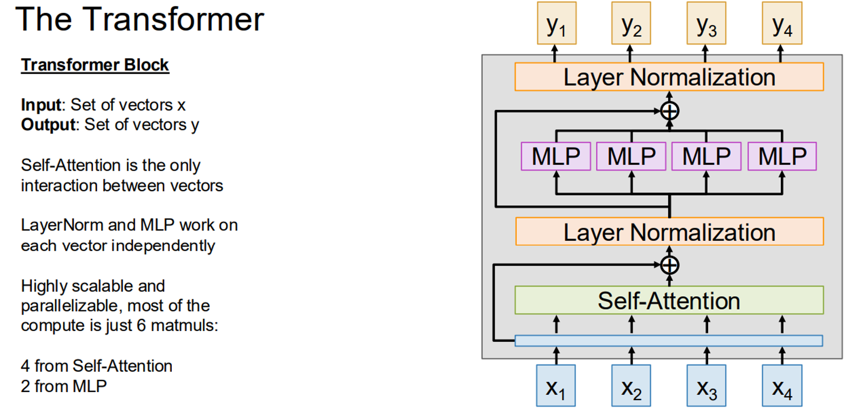
Transformers, introduced in the seminal paper “Attention is All You Need” (Vaswani et al., 2017), rely entirely on attention mechanisms, eliminating the need for RNNs. A transformer block consists of:
- Self-Attention: Allows each input vector to attend to all others, capturing dependencies.
- Layer Normalization: Normalizes each vector independently to stabilize training.
- Multi-Layer Perceptron (MLP): Applies feedforward transformations to each vector.
- Residual Connections: Add the input to the output of each sub-layer to improve gradient flow.
Transformers are highly parallelizable and scalable, with most computation coming from six matrix multiplications (four from self-attention, two from the MLP). Their architecture has remained largely unchanged since 2017 but has scaled significantly in size (e.g., GPT-3 with 175B parameters).
Here’s a PyTorch implementation of a transformer block:
class TransformerBlock(nn.Module):
    def __init__(self, d_model, nhead, dim_feedforward):
        super(TransformerBlock, self).__init__()
        self.self_attention = nn.MultiheadAttention(d_model, nhead)
        self.norm1 = nn.LayerNorm(d_model)
        self.mlp = nn.Sequential(
            nn.Linear(d_model, dim_feedforward),
            nn.ReLU(),
            nn.Linear(dim_feedforward, d_model)
        )
        self.norm2 = nn.LayerNorm(d_model)

    def forward(self, x):
        # Self-Attention
        attn_output, _ = self.self_attention(x, x, x)
        x = self.norm1(x + attn_output)  # Residual connection
        # MLP
        mlp_output = self.mlp(x)
        x = self.norm2(x + mlp_output)  # Residual connection
        return x

# Example usage
transformer_block = TransformerBlock(d_model=512, nhead=8, dim_feedforward=2048)
x = torch.randn(50, 32, 512)  # [seq_len, batch_size, d_model]
output = transformer_block(x)
print(output.shape)  # torch.Size([50, 32, 512])
This code implements a transformer block with self-attention, layer normalization, and an MLP, connected via residual connections.
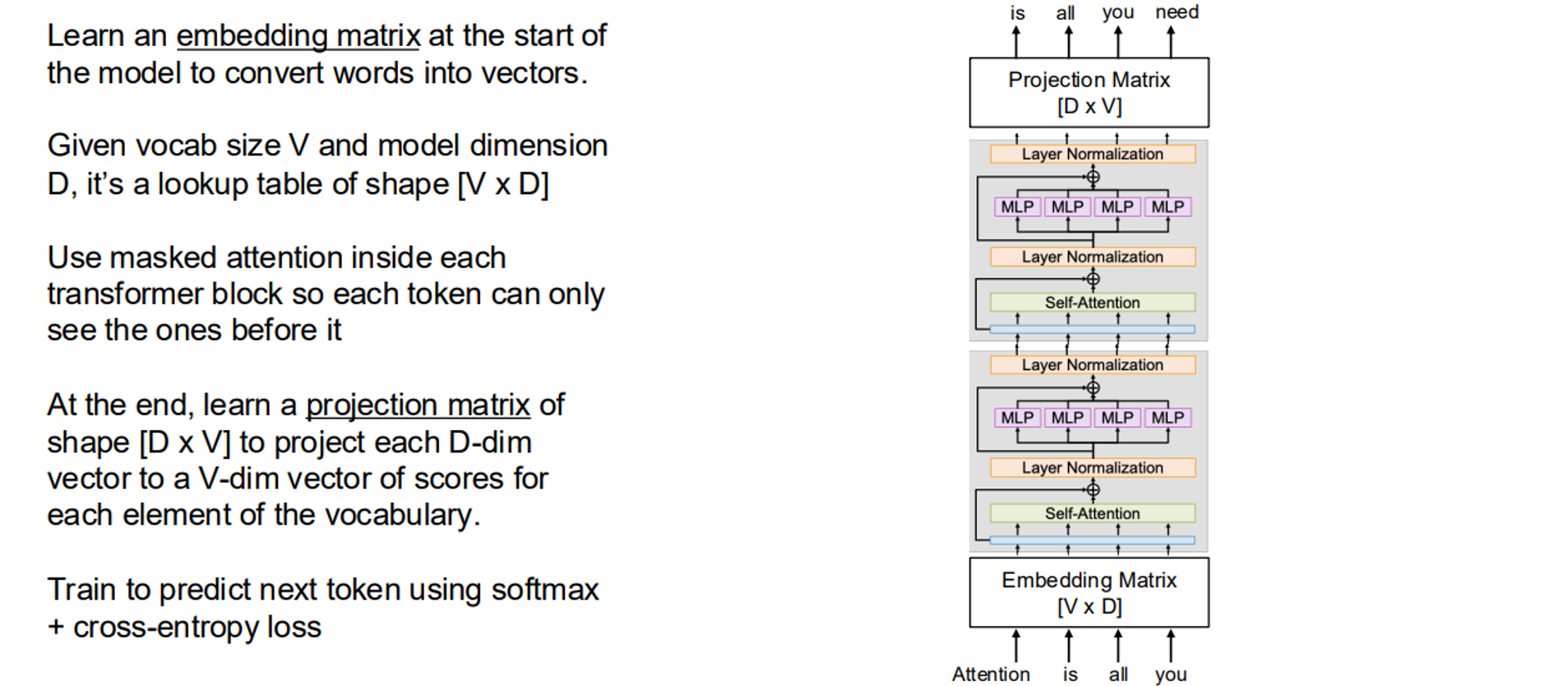
5. Transformers for Language Modeling
Transformers for language modeling (LLMs) convert words into vectors using an embedding matrix, apply masked self-attention to ensure each token only attends to previous tokens, and project the final vectors to vocabulary scores for next-token prediction.
Here’s a simplified PyTorch implementation:
class LanguageModelTransformer(nn.Module):
    def __init__(self, vocab_size, d_model, nhead, num_layers):
        super(LanguageModelTransformer, self).__init__()
        self.embedding = nn.Embedding(vocab_size, d_model)
        self.transformer = nn.Transformer(d_model, nhead, num_layers)
        self.fc = nn.Linear(d_model, vocab_size)

    def forward(self, x):
        x = self.embedding(x)  # [batch_size, seq_len, d_model]
        x = x.permute(1, 0, 2)  # [seq_len, batch_size, d_model]
        mask = nn.Transformer.generate_square_subsequent_mask(x.size(0))
        x = self.transformer(x, x, src_mask=mask)
        x = x.permute(1, 0, 2)  # [batch_size, seq_len, d_model]
        x = self.fc(x)  # [batch_size, seq_len, vocab_size]
        return x

# Example usage
model = LanguageModelTransformer(vocab_size=10000, d_model=512, nhead=8, num_layers=6)
x = torch.randint(0, 10000, (32, 50))  # Batch of 32 sequences
output = model(x)
print(output.shape)  # torch.Size([32, 50, 10000])
This model uses masked attention to predict the next token in a sequence, trained with cross-entropy loss.
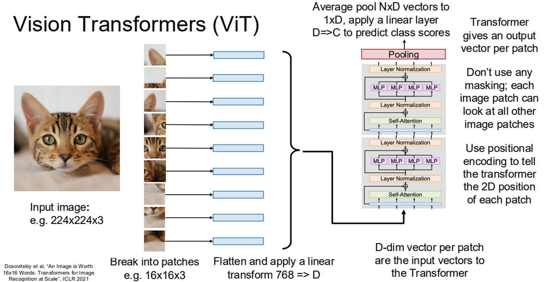
6. Vision Transformers (ViT)
Vision Transformers (ViT) apply transformers to images by dividing them into patches, flattening each patch into a vector, and processing them with a transformer. Positional encodings are added to retain spatial information, and no masking is used, allowing each patch to attend to all others.
Here’s a ViT implementation in PyTorch:
class ViT(nn.Module):
    def __init__(self, image_size, patch_size, num_classes, d_model, nhead, num_layers):
        super(ViT, self).__init__()
        num_patches = (image_size // patch_size) ** 2
        patch_dim = patch_size * patch_size * 3  # Assuming RGB images
        self.patch_embedding = nn.Linear(patch_dim, d_model)
        self.pos_embedding = nn.Parameter(torch.randn(1, num_patches, d_model))
        self.transformer = nn.Transformer(d_model, nhead, num_layers)
        self.fc = nn.Linear(d_model, num_classes)

    def forward(self, x):
        # x: [batch_size, 3, image_size, image_size]
        batch_size = x.size(0)
        x = x.unfold(2, self.patch_size, self.patch_size).unfold(3, self.patch_size, self.patch_size)
        x = x.permute(0, 2, 3, 1, 4, 5).reshape(batch_size, -1, self.patch_size * self.patch_size * 3)
        x = self.patch_embedding(x)  # [batch_size, num_patches, d_model]
        x = x + self.pos_embedding
        x = x.permute(1, 0, 2)  # [num_patches, batch_size, d_model]
        x = self.transformer(x, x)
        x = x.mean(dim=0)  # Average pool
        x = self.fc(x)
        return x

# Example usage
vit = ViT(image_size=224, patch_size=16, num_classes=10, d_model=512, nhead=8, num_layers=6)
x = torch.randn(32, 3, 224, 224)
output = vit(x)
print(output.shape)  # torch.Size([32, 10])
This ViT splits images into patches, embeds them, adds positional encodings, and processes them with a transformer.
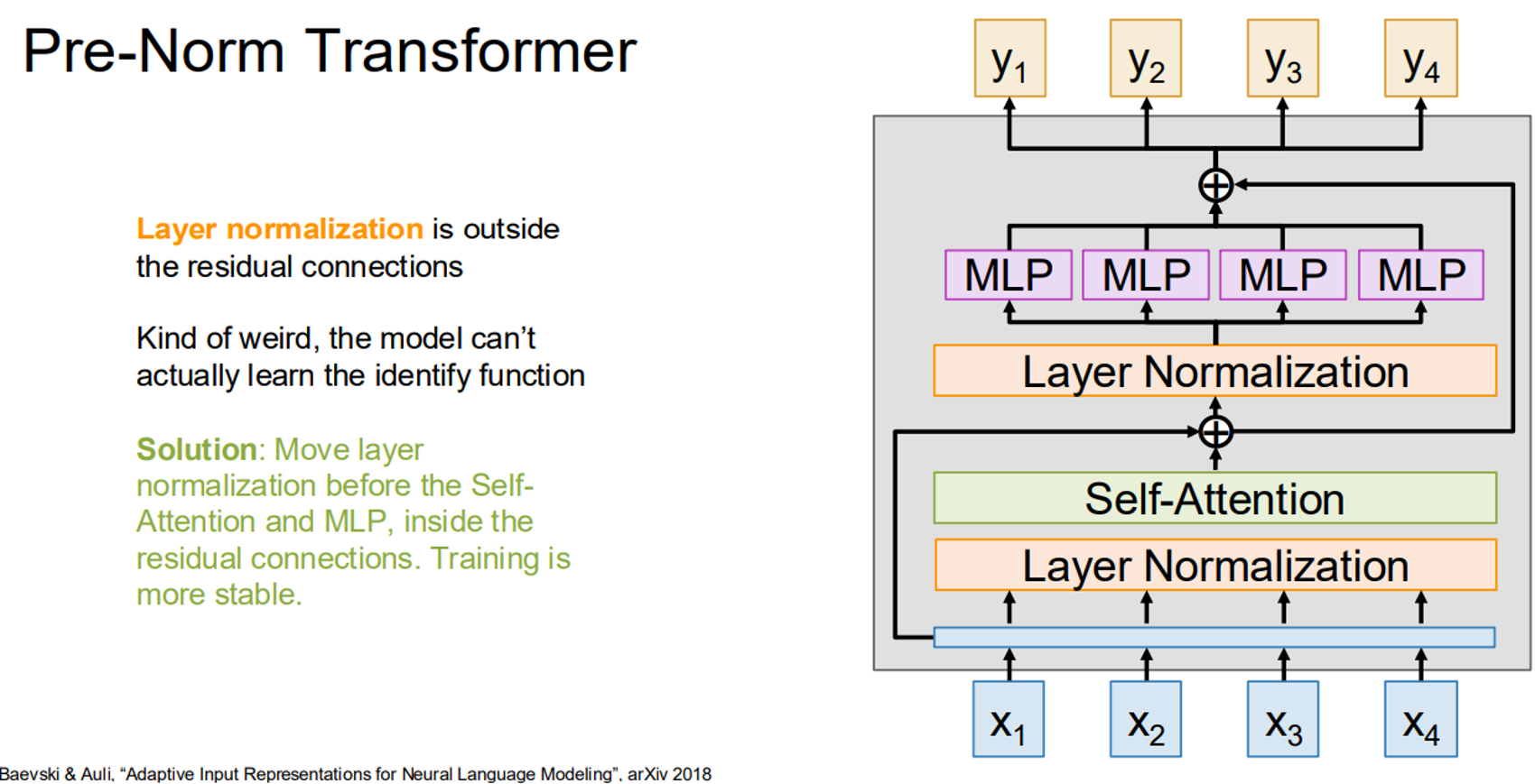
7. Pre-Norm Transformer
In the original transformer, layer normalization is applied after the self-attention and MLP sub-layers, outside the residual connections. Pre-Norm moves normalization inside the residual connections, before the sub-layers, improving training stability.
Here’s a modified transformer block with Pre-Norm:
class PreNormTransformerBlock(nn.Module):
    def __init__(self, d_model, nhead, dim_feedforward):
        super(PreNormTransformerBlock, self).__init__()
        self.norm1 = nn.LayerNorm(d_model)
        self.self_attention = nn.MultiheadAttention(d_model, nhead)
        self.norm2 = nn.LayerNorm(d_model)
        self.mlp = nn.Sequential(
            nn.Linear(d_model, dim_feedforward),
            nn.ReLU(),
            nn.Linear(dim_feedforward, d_model)
        )

    def forward(self, x):
        # Pre-Norm Self-Attention
        x_norm = self.norm1(x)
        attn_output, _ = self.self_attention(x_norm, x_norm, x_norm)
        x = x + attn_output  # Residual connection
        # Pre-Norm MLP
        x_norm = self.norm2(x)
        mlp_output = self.mlp(x_norm)
        x = x + mlp_output  # Residual connection
        return x

# Example usage
pre_norm_block = PreNormTransformerBlock(d_model=512, nhead=8, dim_feedforward=2048)
x = torch.randn(50, 32, 512)
output = pre_norm_block(x)
print(output.shape)  # torch.Size([50, 32, 512])
This block applies normalization before the sub-layers, enhancing stability.
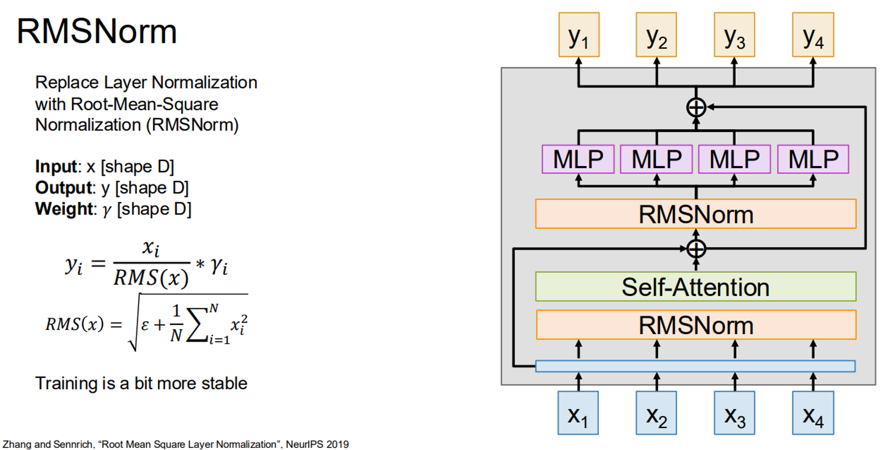
8. RMSNorm
Root-Mean-Square Normalization (RMSNorm) is a simpler alternative to layer normalization, normalizing inputs by their root-mean-square value:
, where .
Here’s an RMSNorm implementation:
class RMSNorm(nn.Module):
    def __init__(self, d_model, eps=1e-6):
        super(RMSNorm, self).__init__()
        self.eps = eps
        self.gamma = nn.Parameter(torch.ones(d_model))

    def forward(self, x):
        rms = torch.sqrt(self.eps + torch.mean(x**2, dim=-1, keepdim=True))
        x = x / rms * self.gamma
        return x

# Example usage
rmsnorm = RMSNorm(d_model=512)
x = torch.randn(32, 50, 512)
output = rmsnorm(x)
print(output.shape)  # torch.Size([32, 50, 512])
RMSNorm is computationally lighter and often more stable than layer normalization.
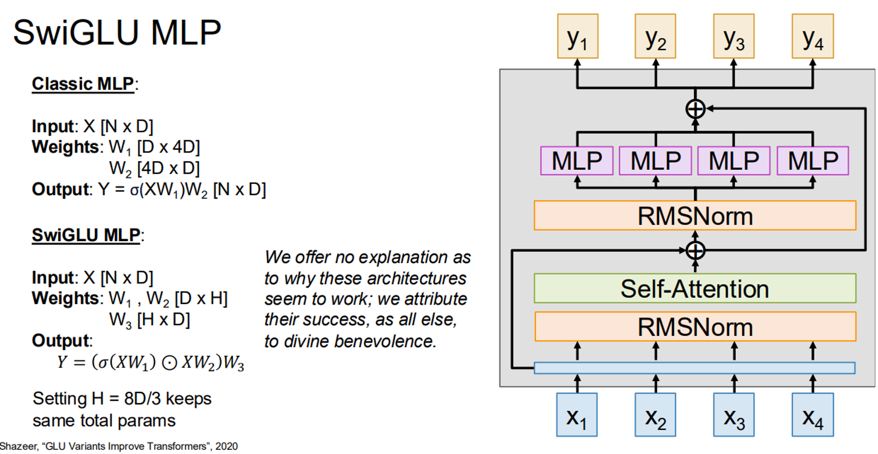
9. SwiGLU MLP
SwiGLU (Swish-Gated Linear Unit) is an advanced MLP variant that uses two weight matrices and a gating mechanism to improve performance:
, where is the Swish activation and is element-wise multiplication.
Here’s a PyTorch implementation:
class SwiGLU(nn.Module):
    def __init__(self, d_model, hidden_dim):
        super(SwiGLU, self).__init__()
        self.w1 = nn.Linear(d_model, hidden_dim)
        self.w2 = nn.Linear(d_model, hidden_dim)
        self.w3 = nn.Linear(hidden_dim, d_model)
        self.swish = lambda x: x * torch.sigmoid(x)

    def forward(self, x):
        gate = self.swish(self.w1(x))
        x = gate * self.w2(x)
        x = self.w3(x)
        return x

# Example usage
swiglu = SwiGLU(d_model=512, hidden_dim=1365)  # 8D/3 ≈ 1365 for same params
x = torch.randn(32, 50, 512)
output = swiglu(x)
print(output.shape)  # torch.Size([32, 50, 512])
SwiGLU enhances the MLP’s expressiveness with a gating mechanism.
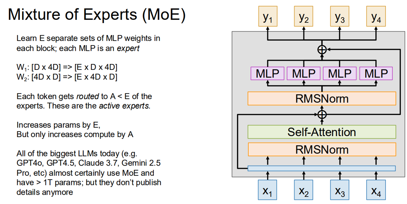
10. Mixture of Experts (MoE)
MoE architectures use multiple MLP “experts” per transformer block, routing each token to a subset of experts. This increases the parameter count significantly while keeping compute costs modest.
Here’s a simplified MoE implementation:
class MoE(nn.Module):
    def __init__(self, d_model, hidden_dim, num_experts, num_active):
        super(MoE, self).__init__()
        self.experts = nn.ModuleList([nn.Sequential(
            nn.Linear(d_model, hidden_dim),
            nn.ReLU(),
            nn.Linear(hidden_dim, d_model)
        ) for _ in range(num_experts)])
        self.gate = nn.Linear(d_model, num_experts)
        self.num_active = num_active

    def forward(self, x):
        # Gating
        gate_scores = torch.softmax(self.gate(x), dim=-1)  # [batch_size, seq_len, num_experts]
        topk_scores, topk_indices = gate_scores.topk(self.num_active, dim=-1)
        topk_scores = torch.softmax(topk_scores, dim=-1)  # Normalize active experts

        # Compute expert outputs
        outputs = torch.zeros_like(x)
        for i in range(self.num_active):
            expert_idx = topk_indices[..., i]  # [batch_size, seq_len]
            expert_output = torch.stack([self.experts[idx](x[b, t])
                                        for b, t, idx in zip(*torch.where(topk_indices == topk_indices))])
            outputs += topk_scores[..., i].unsqueeze(-1) * expert_output
        return outputs

# Example usage
moe = MoE(d_model=512, hidden_dim=2048, num_experts=8, num_active=2)
x = torch.randn(32, 50, 512)
output = moe(x)
print(output.shape)  # torch.Size([32, 50, 512])
This MoE routes each token to two of eight experts, balancing compute and parameter growth.
11. Summary of Transformers
Transformers have become the backbone of large-scale AI models due to their attention-based architecture, which is highly parallelizable and scalable. Key advancements include:
- Pre-Norm: Moving normalization inside residual connections.
- RMSNorm: A simpler, more stable normalization method.
- SwiGLU: A gated MLP for better performance.
- MoE: Multiple experts for increased capacity with modest compute cost.
Transformers are used in language models (e.g., GPT-3), vision tasks (e.g., ViT), and beyond, powering modern AI applications.
Conclusion
Transformers have transformed deep learning by leveraging attention mechanisms to process sequences and sets efficiently. From their roots in NLP to their expansion into vision and other domains, transformers continue to evolve with innovations like Pre-Norm, RMSNorm, SwiGLU, and MoE. The provided PyTorch implementations demonstrate how these concepts can be applied, offering a practical starting point for building transformer-based models.
For further exploration, the next topic in the lecture series is self-supervised learning, which complements transformers in modern AI systems.