Linear Regression Uncertainty Simulation.

Outline

Introduction to the Normal Equation:

• Explains the mathematical formula for computing the regression coefficients analytically:
  $\beta = (X^TX)^{-1} X^T y$.
• Describes the components of the equation, such as the input features matrix ($X$), output values vector ($y$), and the coefficients vector ($\beta$).

Data Generation and Visualization:

• Generates synthetic linear data with and without random noise for demonstration.
• Visualizes the data points and the fitted regression line.

Simulation of Random Noise:

• Simulates the effect of random noise (residuals) on the regression coefficients by running multiple iterations.
• Observes the variability in the coefficients due to noise.

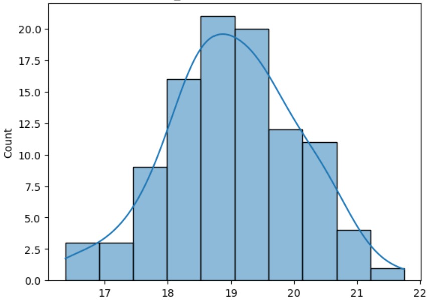
Coefficient Distributions:

• Plots the distributions of the regression coefficients (intercept and slope) across multiple simulations.
• Highlights the uncertainty in the coefficient estimates.

Prediction Uncertainty:

• Simulates predictions at specific input values (e.g., $x=5$) and visualizes the distribution of predictions.
• Computes key percentiles (P10, P50, P90) to summarize prediction uncertainty.

Overall Uncertainty:

• Combines model uncertainty (from coefficient variability) and data uncertainty (from random noise) to estimate total prediction uncertainty.