(Adopted from MIT 6.S191)

Tutorial: Understanding Variational Autoencoders (VAEs)

Variational Autoencoders (VAEs) are one of the most important foundations of modern Generative AI. They combine the strengths of classical autoencoders with probabilistic modeling to create smooth, meaningful latent spaces from which new data samples can be generated.

This tutorial builds upon your knowledge of autoencoders and introduces why they fail as generative models, how VAEs solve the problem, and what key ideas like KL divergence and reparameterization mean in practice.

---

1. Recap: Autoencoders

An autoencoder (AE) is a neural network that learns to:

• Encode data $x$ into a low-dimensional latent representation $z$.
• Decode $z$ back into a reconstruction $\hat{x}$.

The training objective is to minimize reconstruction error:

This makes autoencoders excellent at compression and denoising, but not necessarily at generation.

---

2. Why Autoencoders Fail at Sampling

If you sample a random latent vector $z \sim \mathcal{N}(0, I)$ and pass it through the decoder:

• The output looks like garbage.
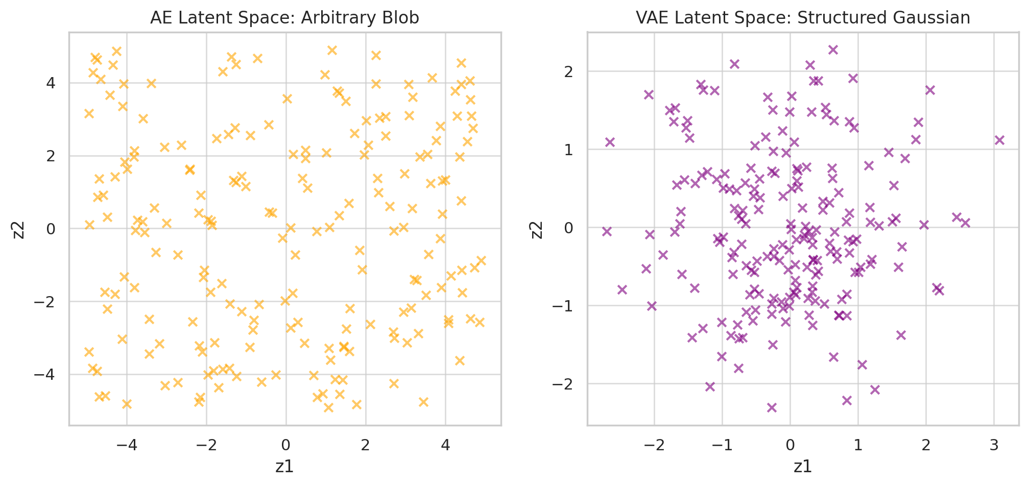
• Reason: the AE only learns to map inputs to some tangled latent blob without ensuring that it aligns with any known probability distribution.

Visual intuition:

• The data manifold is like a narrow road in latent space.
• Autoencoder latents cluster somewhere in space, but not in a structured way.
• Random $z$ lands off-road → decoder has never seen such $z$ → nonsense.

---

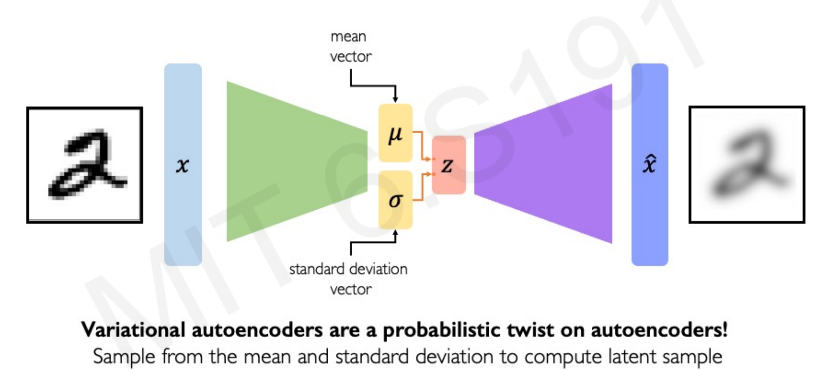
3. Variational Autoencoder (VAE)

VAEs fix this by adding probabilistic structure to the latent space. The idea is:

1. Assume a prior distribution on latents (usually standard Gaussian $p(z) = \mathcal{N}(0, I)$).
2. Force the encoder’s posterior distribution $q_\phi(z|x)$ to be close to this prior.

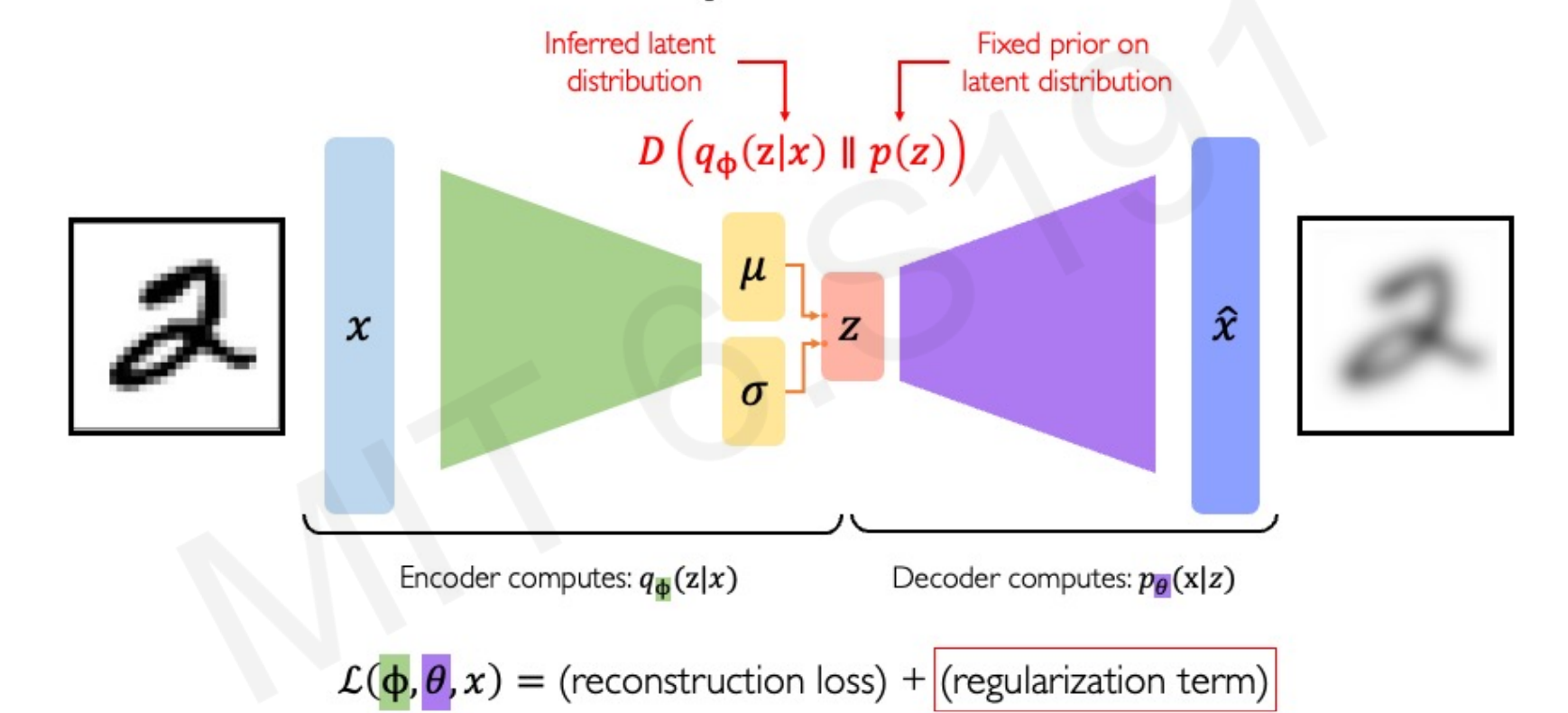
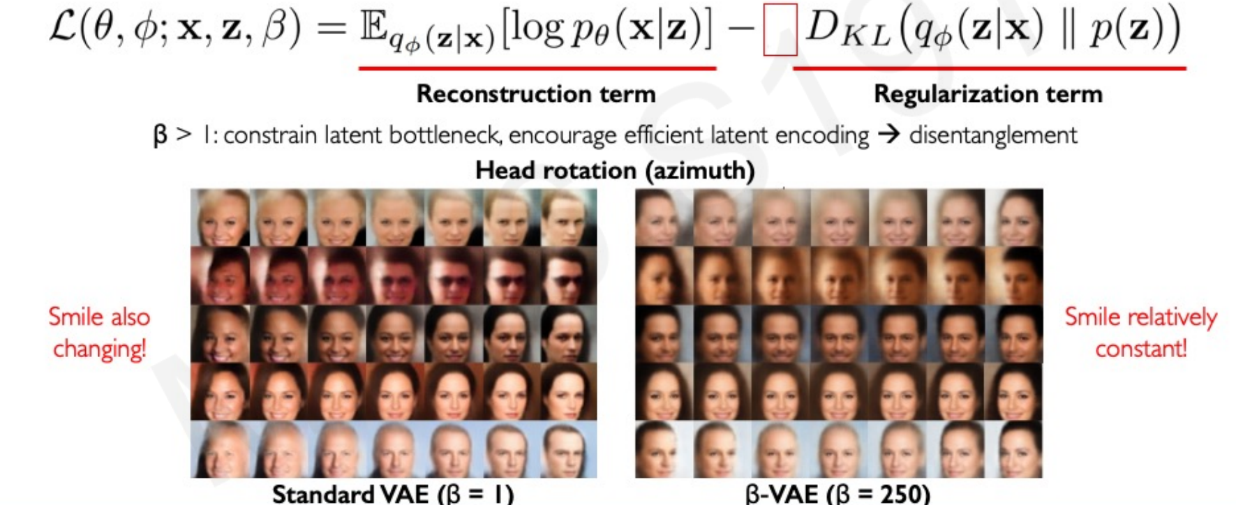
Objective function:

• First term: reconstruction (like AE).
• Second term: regularization, keeps latent space well-behaved.

---

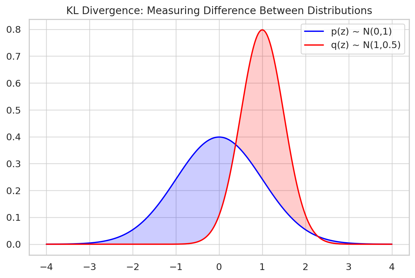
4. KL Divergence

The Kullback–Leibler (KL) divergence) measures how one distribution differs from another:

In VAEs:

• $q(z|x)$: encoder’s output distribution.
• $p(z)$: prior (e.g., Gaussian).

The KL penalty ensures that latent codes are not arbitrary blobs, but instead form a smooth, continuous space aligned with the Gaussian prior.

5. Reparameterization Trick

Problem: Sampling $z \sim q_\phi(z|x)$ is non-differentiable, blocking backpropagation. Solution: Reparameterization trick:

Instead of sampling directly:

We sample:

This makes $z$ a differentiable function of $\mu, \sigma$, enabling gradient descent.

---

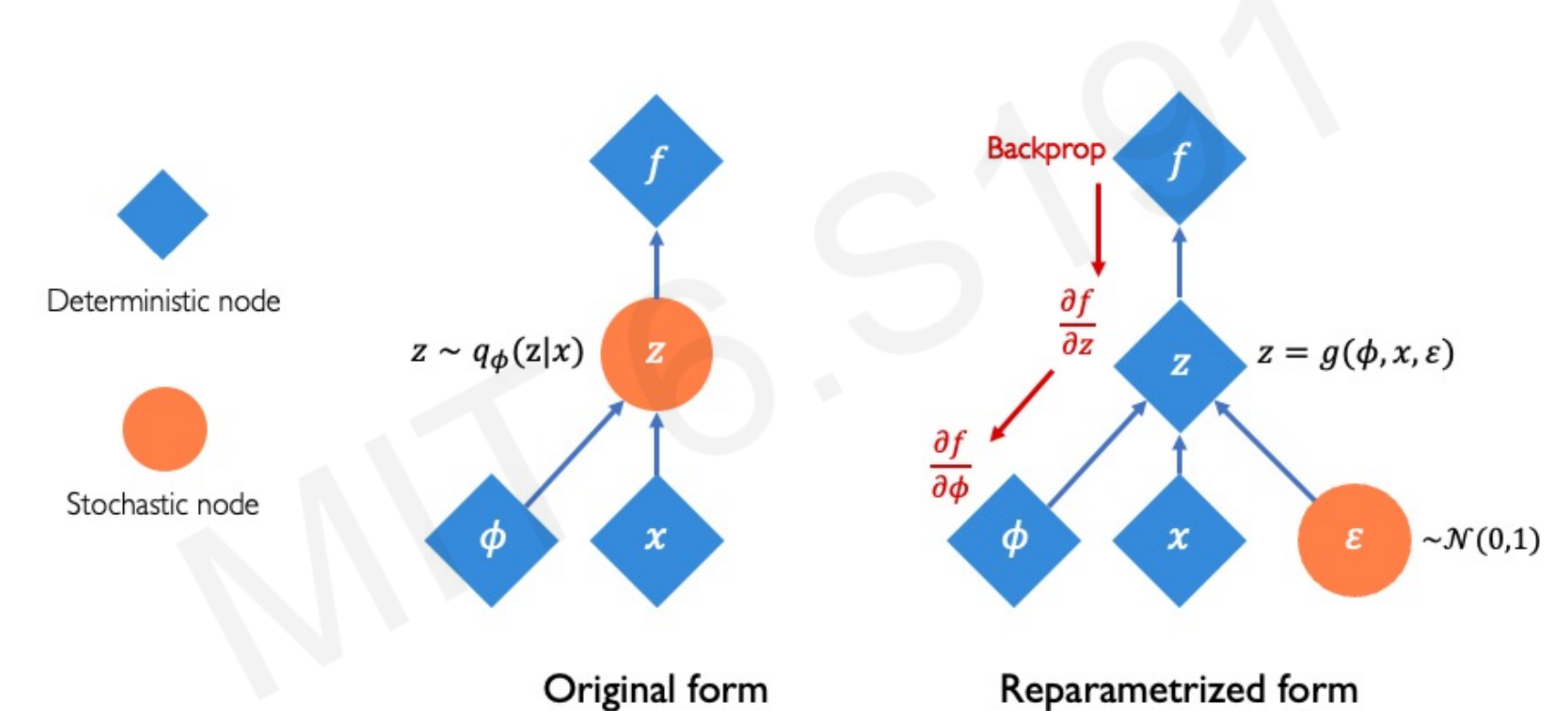
6. VAE Computation Graph

1. Encoder: maps $x \to (\mu, \sigma)$.
2. Reparameterization: sample $z = \mu + \sigma \epsilon$.
3. Decoder: maps $z \to \hat{x}$.
4. Loss: reconstruction + KL regularization.

---

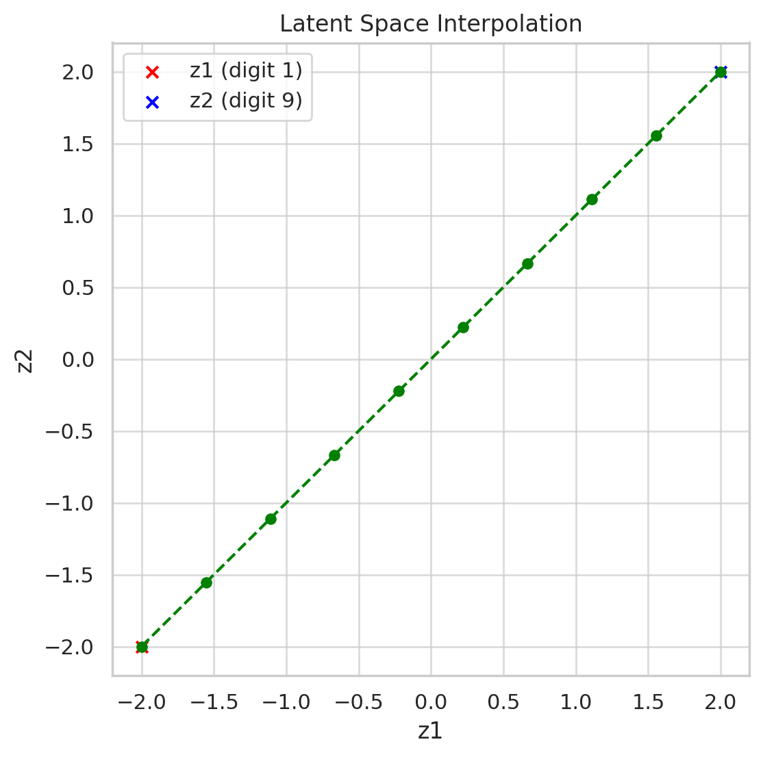
7. Sampling and Latent Perturbations

• Once trained, you can sample $z \sim \mathcal{N}(0,I)$ and decode to get new, realistic samples.
• You can also perturb $z$ slightly to explore variations of data.
• Smooth latent space = meaningful interpolations (e.g., morphing between two images).

---

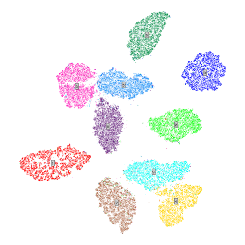
8. AE vs VAE Latent Spaces

📊 Comparison: Autoencoder vs VAE Latent Spaces

9. Disentanglement with β-VAE

• β-VAE introduces a scaling factor $\beta > 1$ on the KL term:

• Effect: stronger regularization → encourages disentangled features (separate factors of variation).

---

10. Python Example: Simple VAE in PyTorch

import torch
import torch.nn as nn
import torch.nn.functional as F

class VAE(nn.Module):
    def __init__(self, input_dim=784, hidden_dim=400, latent_dim=20):
        super().__init__()
        # Encoder
        self.fc1 = nn.Linear(input_dim, hidden_dim)
        self.fc_mu = nn.Linear(hidden_dim, latent_dim)
        self.fc_logvar = nn.Linear(hidden_dim, latent_dim)
        # Decoder
        self.fc2 = nn.Linear(latent_dim, hidden_dim)
        self.fc3 = nn.Linear(hidden_dim, input_dim)

    def encode(self, x):
        h = F.relu(self.fc1(x))
        return self.fc_mu(h), self.fc_logvar(h)

    def reparameterize(self, mu, logvar):
        std = torch.exp(0.5 * logvar)
        eps = torch.randn_like(std)
        return mu + eps * std

    def decode(self, z):
        h = F.relu(self.fc2(z))
        return torch.sigmoid(self.fc3(h))

    def forward(self, x):
        mu, logvar = self.encode(x)
        z = self.reparameterize(mu, logvar)
        return self.decode(z), mu, logvar

# Loss function
def vae_loss(recon_x, x, mu, logvar):
    recon_loss = F.binary_cross_entropy(recon_x, x, reduction='sum')
    kl = -0.5 * torch.sum(1 + logvar - mu.pow(2) - logvar.exp())
    return recon_loss + kl

---

11. Summary

• Plain autoencoders fail at sampling because latent space is unstructured.
• VAEs introduce probabilistic latent variables with a Gaussian prior.
• The KL divergence aligns the latent posterior with the prior.
• The reparameterization trick enables differentiable sampling.
• Extensions like β-VAE improve disentanglement of latent features.

---